Space as a scaffold for rotational generalisation of abstract concepts
Figures
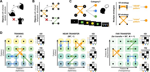
Paradigm.
(A) Objects can be perceived as similar despite changes in shape, orientation, and features. (B) Similarly, can sequences of features be perceived as similar despite great changes in the features that composed them? (C) In our experiments, participants had to learn the category associated with quadruplets composed of four stimuli drawn from a 2D feature manifold. To do so, they could use one of two major strategies: tracking changes in a single dimension (1D) or two dimensions (2D). (D) Illustration of the feature manifold and transition vectors in the visual modality. Each transition vector defined transitions between cardinally or diagonally adjacent features on a 2D manifold (here, given by colour and spikiness for training and near transfer in the left and middle panels, and by transparency and squareness in the far transfer condition). The transition vectors for each category are shown in their canonical (0°) rotation as blue, orange, and green arrows superimposed on each feature manifold. The vectors are shown rotated by 90° in the near and far transfer conditions. Next to each feature manifold is a matrix showing the expected mapping (filled squares) from feature vectors to categories for a participant using the 1D strategies (top and middle) and 2D strategy (bottom). Note that the 2D strategy always leads to effective generalisation (rotated exemplars are mapped on their corresponding categories) even in transfer, as indicated by filled squares on the matrix diagonal, whereas a 1D strategy leads to a different pattern. We use the symbols ∅, ↶, and ★ to denote canonical (0°), 90° rotation, and far transfer conditions, respectively.
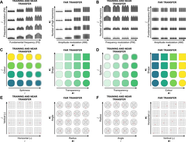
Examples of 2D feature manifolds used in the study.
For each modality, four manifolds are displayed. (A, B) In the auditory modality, the stimuli could vary along four features: fundamental frequency F0 (110, 220, 330, or 440 Hz), frequency modulation (1, 2, 3, or 4 Hz), amplitude modulation (1, 2, 3, or 4 Hz), and number of high harmonics (1, 3, 7, or 10). A spectrogram of each sound is displayed at its location on the manifold. Two example sets of original and far transfer manifolds corresponding to the manifolds of two different participants are shown in A and B. (C, D) In the visual modality, the stimuli could vary along four features: colour (viridis perceptually uniform colormap, 0, 0.33, 0.66, or 1), transparency level (0.2, 0.46, 0.73, or 1), squareness (squareness parameter of the Fernandez-Guasti squircle, 0.01, 0.8, 0.98, or 1), and spikiness (amplitude of the cosine modulation relative to the squircle radius, 0, 0.06, 0.13, or 0.2). Two example sets of original and far transfer manifolds corresponding to the manifolds of two different participants are shown in C and D. (E, F) In the spatial modality, the stimuli could vary along four features: horizontal position (1, 2, 3, or 4), vertical position (1, 2, 3, or 4), radius (1, 2, 3, or 4), and angle (0, 90°, 180°, or 270°). Two example sets of original and far transfer manifolds corresponding to the manifolds of two different participants are shown in E and F.
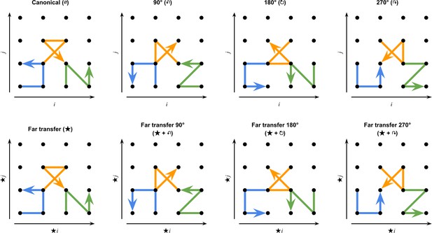
The eight transformations of the canonical quadruplets present in the study.
There are three categories of quadruplets, shown in three different colours. Eight transformations have been used: canonical (∅), 90° rotation (↶), 180° rotation (↻), 270° rotation (↷), far transfer canonical (★), far transfer 90° rotation (★ + ↶), far transfer 180° rotation (★ + ↻), and far transfer 270° rotation (★ + ↷).

Example trials.
(A) Example trial of the main quadruplet categorisation task. Participants were asked to infer the category of quadruplets, e.g., here four visual shapes that vary in colour and spikiness. Participants gave their response by clicking on one of the three buttons that appeared on screen after the presentation of the quadruplets. Participants received trialwise and blockwise feedback on training trials (see Materials and methods for details). (B) Example trial of the mapping task. Participants were asked to associate features from different modalities, e.g., here map individual visual images to their corresponding location in physical space. Participants gave their response by clicking on a location on a 4×4 grid that appeared on screen after the presentation of the stimulus. Participants received trialwise and blockwise feedback. (C) Example trial of the duration-match filler task used in Exp. 4. Participants were asked to infer the category of sequences, defined by the number of blue stars in a sequence of four stationary stars. Participants gave their response by clicking on one of the three buttons that appeared on screen after the presentation of the sequence (the buttons were different between the main task and the filler task). Participants received trialwise and blockwise feedback.
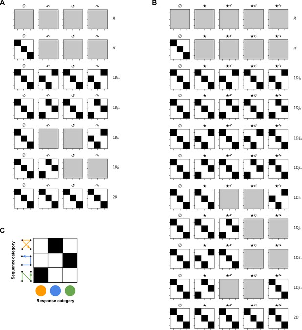
Model response matrices to the different quadruplets transformations in Experiment 1.
(A) Near transfer. The degree of fading indicates the probability of a response (white to black: 0–1). (B) Far transfer. (C) This example response matrix reads as follows: a model with this response matrix would respond ‘orange’ when presented with a ‘category 2’ (the ‘z’ shape) quadruplet. In Exp. 1, feedback was given only on canonical (0°, denoted by ∅) trials.
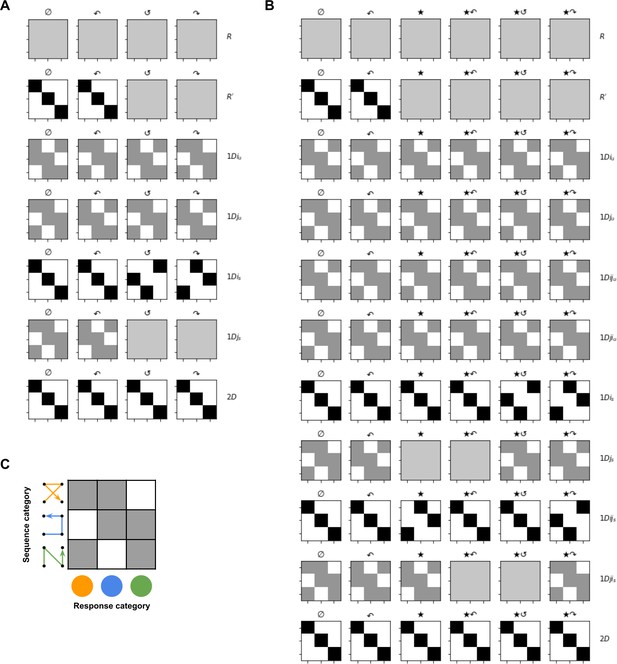
Model response matrices to the different quadruplets transformations in Experiment 2, 3, and 4.
(A) Near transfer. The degree of fading indicates the probability of a response (white to black: 0–1). (B) Far transfer. (C) This example response matrix reads as follows: a model with this response matrix would respond 50% of the time ‘orange’ and 50% of the time ‘green’ when presented with a ‘category 2’ (the ‘z’ shape) quadruplet. In Exp. 2, 3, and 4, feedback was given on canonical (0°, denoted by ∅) and 90° (↶) trials.
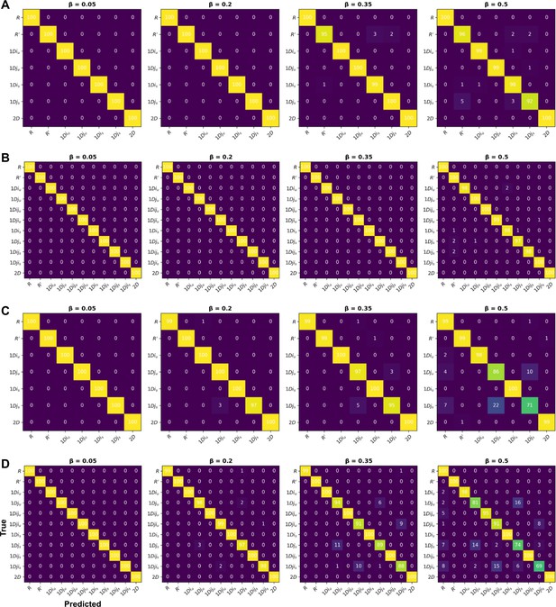
Model recovery analysis.
Synthetic data were generated using the same trials as the participants for all models. This analysis was repeated 100 times for four level of the temperature parameter (β=0.05, 0.2, 0.35, and 0.5). (A) Near transfer in Exp. 1. (B) Far transfer in Exp. 1. (C) Near transfer in Exp. 2, 3, and 4. (D) Far transfer in Exp. 2, 3, and 4.

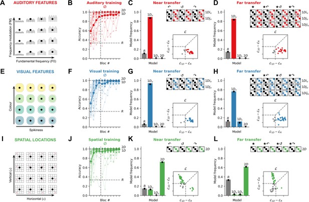
Experiment 1: Quadruplets composed of spatial locations, but not auditory or visual features, are associated with a 2D strategy.
(A) In the auditory modality (N=50), the 2D feature manifold was defined by auditory features. Here, we illustrate with a schematic in which the feature manifold is defined by fundamental frequency and frequency modulation. (B) Accuracy on training trials involving the canonical transition vectors (0° rotation, denoted by the symbol ∅). The bold curve and dots represent the group average; lighter curves are individual participants. During training, random models (R) are at chance (33% accuracy; lower dashed line), while idealised 1D and 2D models are at ceiling (100% accuracy; upper dashed lines). (C) Model fits to the near transfer responses. The bar plot shows model frequencies in the population and black dots are Bayesian point estimates of the model frequency. The matrices show cross-validated model predictions in the same format at Figure 1D, except with the degree of fading (light to dark colour) signalling average participant responses in each case. The matrices read as follows: the top row depicts the average behaviour of participants who were best fit by the 1Diu model (using a held-out set of responses). The 1Diu model predictions are shown in black for three rotations of the quadruplets (90°, 180°, 270° denoted by the symbols ↶, ↺, and ↷ respectively). The average response matrices of the participants using held-out responses are shown in red. The scatter plot below shows individual likelihoods for the 1D and 2D models (normalised by the R model). Each dot is an individual participant, coded by whether they are best fit by either 1D or 2D models (colour) or the R model (grey). Dashed lines distinguish zones of relative likelihood where participants are best fit by R (bottom left square), 1D (rightmost quadrilateral), or 2D (upper quadrilateral) models. (D) Model fits to the far transfer responses, using the same conventions as C. Note that, at transfer, more 1D models are possible because of the differing ways that participants could map between the i and j axes and the ★i and ★j axes during training and far transfer. (E) In the visual modality (N=52), the 2D feature manifold was defined by visual attributes; here we use colour and spikiness as an illustration. (F–H) depict data from the visual modality using conventions from B–D. (I) In the spatial modality (N=51), the 2D feature manifold was defined by the spatial location of a star (here a red dot is used for illustration). (J–L) depict data from the spatial modality using conventions from B–D.
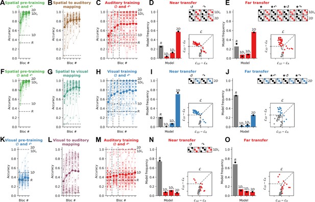
Experiment 2: Spatial pre-training triggers the use of a 2D strategy for quadruplets composed of auditory or visual features.
(A) Performance on the spatial pre-training task in Exp. 2a (N=51). For this and all plots below, the bold line is the group average and lighter lines are individual participants. Dashed lines show expected average performance under the corresponding models (labelled). (B) Performance in the spatial to auditory mapping task. Chance performance is at 1/16 (dashed line). (C) Performance on training trials in the auditory modality for canonical (0°) and 90° rotated quadruplets. During training, random models (R) are at chance (33% accuracy), almost all 1D models are at 50% accuracy, and 1Dis and 2D models are at ceiling (100% accuracy). (D) Model fits to the near transfer responses, using the same conventions as Figure 2. Model predictions are shown in black for two rotations of the quadruplets (180° and 270° denoted by the symbols ↺ and ↷, respectively). (E) Model fits to the far transfer responses. (F–J) read as A–E for Exp. 2b (N=51), where participants performed a spatial pre-training and a spatial to visual mapping task prior to performing the visual version of the main task. (K–O) read as A–E for Exp. 2c (N=50), where participants performed a visual pre-training and a visual to auditory mapping task prior to performing the auditory version of the main task.
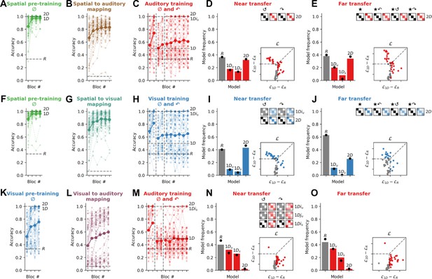
Experiment 3: Exposure to the canonical events (0°) during spatial pre-training is sufficient to trigger the use of a 2D strategy.
All panels use the same conventions as Figure 3. (A–E) Contrary to Exp. 2a, in Exp. 3a (N=50), participants were exposed only to canonical events (0°) during the spatial pre-training. (F–J) Exp. 3b (N=51). (K–O) Exp. 3c (N=50).
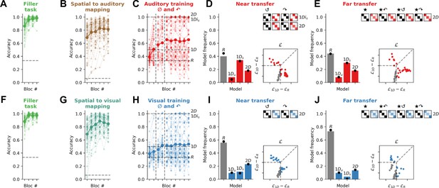
Experiment 4: (A–E).
Contrary to Exp. 3a, in Exp. 4a (N=50), participants were exposed to an irrelevant counting task instead of the spatial pre-training. (F–J) Exp. 3b (N=52). Figure used the same conventions as Figure 4.
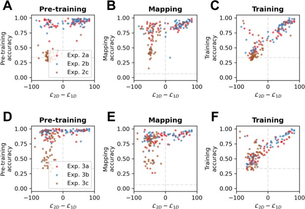
Correlation analysis.
Scatter plots of 2Dness (the difference in likelihood between the best 1D model and the 2D model in the training modality in near transfer) and (A) pre-training accuracy, (B) mapping accuracy, and (C) training accuracy in the testing modality in Exp. 2. Dots are individual participants in Exp. 2a (red), 2b (blue), and 2c (brown). (D–F) read as A–C for Exp. 3.
Results of Exp. 1 when selecting participants that reached > 90% accuracy in the last block of training.
Captions are the same as Figure 2 of the main text.
Tables
Demographic data.
µ: average, σ: standard deviation, F: female, M: male.
| N | Age (µ ± σ) | Sex (F/M/other) | |
|---|---|---|---|
| Exp. 1 | 153 | 29.4±6.1 | 70/68/15 |
| Exp. 2 | 152 | 29.9±5.9 | 88/62/2 |
| Exp. 3 | 151 | 29.4±5.4 | 88/63/0 |
| Exp. 4 | 102 | 28.5±6.1 | 65/37/0 |
| Total | 558 | 29.4±5.9 | 311/230/17 |
Procedure for Experiment 1.
The table reads as follows: on day 1, participants in the Exp. 1a began with 120 trials of the quadruplet categorisation task in the auditory modality, with canonical quadruplets (0°, denoted by ∅), with feedback on every trials. They subsequently performed 105 trials (with trialwise feedback) and 105 transfer trials including rotated and far transfer quadruplets (without trialwise feedback) which were presented in mixed blocks of 30 trials. Training and transfer trials were randomly interleaved, and no clue indicated whether participants were currently on a training trial or a transfer trial before feedback (or absence of feedback in case of a transfer trial). All participants thus performed a total of 330 trials in a single session. Abbreviations/symbols: Fb.: trialwise feedback. Trans.: transformations of the quadruplets. Transformations are canonical (∅), 90° rotation (↶), 180° rotation (↻), 270° rotation (↷), far transfer canonical (★), far transfer 90° rotation (★ + ↶), far transfer 180° rotation (★ + ↻), and far transfer 270° rotation (★ + ↷).
| Day | Task | Trial # | Trans. | Fb. | Exp. 1a(N=50) | Exp. 1b(N=52) | Exp. 1c(N=51) |
|---|---|---|---|---|---|---|---|
| 1 | Quadruplet categorisation | 120 | ∅ | Yes | Auditory | Visual | Spatial |
| Quadruplet categorisation | 105 | ∅ | Yes | Auditory | Visual | Spatial | |
| 105 | ↶ ↻ ↷ ★ ★ + ↶ ★ + ↻ ★ + ↷ | No | Auditory | Visual | Spatial |
Procedure for Experiment 2.
Same as Table 2. All participants thus performed a total of 396 trials on day 1 and 600 trials on day 2. Sp. → Aud.: spatial to auditory mapping task. Sp. → Vis.: spatial to visual mapping task. Vis. → Aud.: visual to auditory mapping task.
| Day | Task | Trial # | Trans. | Fb. | Exp. 2a(N=51) | Exp. 2b(N=51) | Exp. 2c(N=50) |
|---|---|---|---|---|---|---|---|
| 1 | Quadruplet categorisation | 60 | ∅ ↶ | Yes | Spatial | Spatial | Visual |
| Mapping | 48 | i | Yes | Sp. → Aud. | Sp. → Vis. | Vis. → Aud. | |
| 48 | j | Yes | Sp. → Aud | Sp. → Vis. | Vis. → Aud. | ||
| 48 | ij | Yes | Sp. → Aud | Sp. → Vis. | Vis. → Aud. | ||
| Mapping | 48 | i | Yes | Sp. → Aud | Sp. → Vis. | Vis. → Aud. | |
| 48 | j | Yes | Sp. → Aud | Sp. → Vis. | Vis. → Aud. | ||
| 96 | ij | Yes | Sp. → Aud | Sp. → Vis. | Vis. → Aud. | ||
| 2 | Quadruplet categorisation | 60 | ∅ ↶ | Yes | Spatial | Spatial | Visual |
| Mapping | 48 | i | Yes | Sp. → Aud | Sp. → Vis. | Vis. → Aud. | |
| 48 | j | Yes | Sp. → Aud | Sp. → Vis. | Vis. → Aud. | ||
| 48 | ij | Yes | Sp. → Aud | Sp. → Vis. | Vis. → Aud. | ||
| Quadruplet categorisation | 30 | ∅ ↶ | Yes | Sp.+Aud | Sp.+Vis. | Vis.+Aud | |
| 30 | ∅ ↶ | Yes | Auditory | Visual | Auditory | ||
| Mapping | 48 | ij | Yes | Sp. → Aud | Sp. → Vis. | Vis. → Aud | |
| Quadruplet categorisation | 60 | ∅ ↶ | Yes | Auditory | Visual | Auditory | |
| Mapping | 48 | ij | Yes | Sp. → Aud | Sp. → Vis. | Vis. → Aud | |
| Quadruplet categorisation | 90 | ∅ ↶ | Yes | Auditory | Visual | Auditory | |
| 90 | ↻ ↷ ★ ★ + ↶ ★ + ↻ ★ + ↷ | No | Auditory | Visual | Auditory |
Procedure for Experiment 3.
Same conventions as Table 2.
| Day | Task | Trial # | Trans. | Fb. | Exp. 3a(N=50) | Exp. 3b(N=51) | Exp. 3c(N=50) |
|---|---|---|---|---|---|---|---|
| 1 | Quadruplet categorisation | 60 | ∅ | Yes | Spatial | Spatial | Visual |
| Mapping | 48 | i | Yes | Sp. → Aud. | Sp. → Vis. | Vis. → Aud. | |
| 48 | j | Yes | Sp. → Aud | Sp. → Vis. | Vis. → Aud. | ||
| 48 | ij | Yes | Sp. → Aud | Sp. → Vis. | Vis. → Aud. | ||
| Mapping | 48 | i | Yes | Sp. → Aud | Sp. → Vis. | Vis. → Aud. | |
| 48 | j | Yes | Sp. → Aud | Sp. → Vis. | Vis. → Aud. | ||
| 96 | ij | Yes | Sp. → Aud | Sp. → Vis. | Vis. → Aud. | ||
| 2 | Quadruplet categorisation | 60 | ∅ | Yes | Spatial | Spatial | Visual |
| Mapping | 48 | i | Yes | Sp. → Aud | Sp. → Vis. | Vis. → Aud. | |
| 48 | j | Yes | Sp. → Aud | Sp. → Vis. | Vis. → Aud. | ||
| 48 | ij | Yes | Sp. → Aud | Sp. → Vis. | Vis. → Aud. | ||
| Quadruplet categorisation | 30 | ∅ | Yes | Sp.+Aud | Sp.+Vis. | Vis.+Aud | |
| 30 | ∅ ↶ | Yes | Auditory | Visual | Auditory | ||
| Mapping | 48 | ij | Yes | Sp. → Aud | Sp. → Vis. | Vis. → Aud | |
| Quadruplet categorisation | 60 | ∅ ↶ | Yes | Auditory | Visual | Auditory | |
| Mapping | 48 | ij | Yes | Sp. → Aud | Sp. → Vis. | Vis. → Aud | |
| Quadruplet categorisation | 90 | ∅ ↶ | Yes | Auditory | Visual | Auditory | |
| 90 | ↻ ↷ ★ ★ + ↶ ★ + ↻ ★ + ↷ | No | Auditory | Visual | Auditory |
Procedure for Experiment 4.
Same as Table 2.
| Day | Task | Trial # | Trans. | Fb. | Exp. 4a(N=50) | Exp. 4b(N=52) |
|---|---|---|---|---|---|---|
| 1 | Filler | 60 | Yes | Spatial | Spatial | |
| Mapping | 48 | i | Yes | Sp. → Aud. | Sp. → Vis. | |
| 48 | j | Yes | Sp. → Aud | Sp. → Vis. | ||
| 48 | ij | Yes | Sp. → Aud | Sp. → Vis. | ||
| Mapping | 48 | i | Yes | Sp. → Aud | Sp. → Vis. | |
| 48 | j | Yes | Sp. → Aud | Sp. → Vis. | ||
| 96 | ij | Yes | Sp. → Aud | Sp. → Vis. | ||
| 2 | Filler | 60 | ∅ | Yes | Spatial | Spatial |
| Mapping | 48 | i | Yes | Sp. → Aud | Sp. → Vis. | |
| 48 | j | Yes | Sp. → Aud | Sp. → Vis. | ||
| 48 | ij | Yes | Sp. → Aud | Sp. → Vis. | ||
| Quadruplet categorisation | 60 | ∅ ↶ | Yes | Auditory | Visual | |
| Mapping | 48 | ij | Yes | Sp. → Aud | Sp. → Vis. | |
| Quadruplet categorisation | 60 | ∅ ↶ | Yes | Auditory | Visual | |
| Mapping | 48 | ij | Yes | Sp. → Aud | Sp. → Vis. | |
| Quadruplet categorisation | 90 | ∅ ↶ | Yes | Auditory | Visual | |
| 90 | ↻ ↷ ★ ★ + ↶ ★ + ↻ ★ + ↷ | No | Auditory | Visual |
Bayes factors quantifying the support in favour of a difference in model frequencies between each pair of conditions in the near transfer condition: 1D vs 2D.
Models were grouped in two families as follows: [1Diu, 1Dju, 1Dis, 1Djs], [2D]. A BF>1 indicates evidence in favour of a difference in model frequencies (green, BF>3, BF>10, and BF>100 corresponds respectively to substantial, strong, and decisive evidence in favour of a difference in model frequencies between groups). A BF<1 indicates evidence in favour of similar model frequencies (red, BF<0.3, BF<0.1, and BF<0.01 corresponds respectively to substantial, strong, and decisive evidence in favour of no difference in model frequencies between groups).
| Exp. 1b | Exp. 1c | Exp. 2a | Exp. 2b | Exp. 2c | Exp. 3a | Exp. 3b | Exp. 3c | Exp. 4a | Exp. 4b | |
|---|---|---|---|---|---|---|---|---|---|---|
| Exp. 1a | 0.1 | 1.1×10¹⁷ | 4.5×10¹⁰ | 1.0×10¹⁵ | 0.9 | 8.1×10⁴ | 6.6×10⁷ | 0.2 | 85.8 | 730.1 |
| Exp. 1b | 3.8×10⁷ | 1.1×10¹¹ | 3.1×10¹⁵ | 1.0 | 1.2×10⁵ | 1.3×10⁸ | 0.2 | 106.7 | 979.4 | |
| Exp. 1c | 2.0 | 0.2 | 6.3×10¹² | 6999.7 | 40.3 | 2.1×10¹⁵ | 9.6×10⁷ | 4.2×10⁶ | ||
| Exp. 2a | 0.6 | 9.0×10⁶ | 3.4 | 0.3 | 1.2×10⁹ | 1630.6 | 169.8 | |||
| Exp. 2b | 8.3×10¹⁰ | 483.7 | 5.9 | 2.2×10¹³ | 2.6×10⁶ | 1.4×10⁵ | ||||
| Exp. 2c | 122.5 | 3.1×10⁴ | 0.3 | 0.9 | 3.6 | |||||
| Exp. 3a | 0.4 | 4220.0 | 0.9 | 0.3 | ||||||
| Exp. 3b | 2.4×10⁶ | 26.6 | 4.8 | |||||||
| Exp. 3c | 8.6 | 56.0 | ||||||||
| Exp. 4a | 0.2 |
Bayes factors quantifying the support in favour of a difference in model frequencies between each pair of conditions in the near transfer condition: R vs 1D/2D.
Models were grouped in two families as follows: [R, R’], [1Diu, 1Dju, 1Dis, 1Djs, 2D].
| Exp. 1b | Exp. 1c | Exp. 2a | Exp. 2b | Exp. 2c | Exp. 3a | Exp. 3b | Exp. 3c | Exp. 4a | Exp. 4b | |
|---|---|---|---|---|---|---|---|---|---|---|
| Exp. 1a | 1.7 | 17.7 | 2.7 | 9.7 | 7.4 | 0.3 | 0.2 | 0.2 | 0.2 | 0.3 |
| Exp. 1b | 0.2 | 0.2 | 0.2 | 2.1×10⁵ | 0.3 | 0.4 | 0.8 | 0.5 | 20.4 | |
| Exp. 1c | 0.2 | 0.2 | 1.4×10⁶ | 1.0 | 2.3 | 6.1 | 2.7 | 437.0 | ||
| Exp. 2a | 0.2 | 4.0×10⁵ | 0.3 | 0.6 | 1.2 | 0.7 | 36.0 | |||
| Exp. 2b | 4.6×10⁶ | 0.7 | 1.5 | 3.6 | 1.7 | 196.9 | ||||
| Exp. 2c | 198.0 | 47.7 | 13.1 | 34.0 | 0.8 | |||||
| Exp. 3a | 0.2 | 0.2 | 0.2 | 1.3 | ||||||
| Exp. 3b | 0.2 | 0.2 | 0.6 | |||||||
| Exp. 3c | 0.2 | 0.3 | ||||||||
| Exp. 4a | 0.5 |
Bayes factors quantifying the support in favour of a difference in model frequencies between each pair of conditions in the far transfer condition: 1D vs 2D.
Models were grouped in two families as follows: [1Diu, 1Diju, 1Dju, 1Djiu 1Dis, 1Dijs, 1Djs, 1Djis], [2D].
| Exp. 1b | Exp. 1c | Exp. 2a | Exp. 2b | Exp. 2c | Exp. 3a | Exp. 3b | Exp. 3c | Exp. 4a | Exp. 4b | |
|---|---|---|---|---|---|---|---|---|---|---|
| Exp. 1a | 0.1 | 2.0×10¹² | 4.0×10¹⁰ | 3.5×10¹¹ | 1.9 | 3.4×10⁵ | 8.5×10⁵ | 0.4 | 88.7 | 366.1 |
| Exp. 1b | 4.6×10¹² | 8.4×10¹⁰ | 7.6×10¹¹ | 2.1 | 5.1×10⁵ | 1.3×10⁶ | 0.4 | 107.2 | 461.3 | |
| Exp. 1c | 0.2 | 0.2 | 3.6×10⁷ | 7.2 | 4.1 | 2.8×10⁹ | 2.3×10⁴ | 3403.6 | ||
| Exp. 2a | 0.2 | 1.2×10⁶ | 1.5 | 1.0 | 7.3×10⁷ | 1439.1 | 266.4 | |||
| Exp. 2b | 8.0×10⁶ | 3.7 | 2.2 | 5.6×10⁸ | 6820.3 | 1126.7 | ||||
| Exp. 2c | 101.4 | 204.2 | 0.2 | 0.5 | 1.0 | |||||
| Exp. 3a | 0.2 | 1976.8 | 1.6 | 0.7 | ||||||
| Exp. 3b | 4445.1 | 2.6 | 1.0 | |||||||
| Exp. 3c | 2.4 | 6.8 | ||||||||
| Exp. 4a | 0.2 |
Bayes factors quantifying the support in favour of a difference in model frequencies between each pair of conditions in the far transfer condition: R vs 1D/2D.
Models were grouped in two families as follows: [R, R’], [1Diu, 1Diju, 1Dju, 1Djiu, 1Dis, 1Dijs, 1Djs, 1Djis, 2D].
| Exp. 1b | Exp. 1c | Exp. 2a | Exp. 2b | Exp. 2c | Exp. 3a | Exp. 3b | Exp. 3c | Exp. 4a | Exp. 4b | |
|---|---|---|---|---|---|---|---|---|---|---|
| Exp. 1a | 0.5 | 0.2 | 1.2 | 1.4 | 2.7 | 0.3 | 0.6 | 0.2 | 0.2 | 9.6 |
| Exp. 1b | 0.2 | 0.2 | 131.0 | 340.4 | 0.2 | 22.9 | 0.4 | 0.3 | 2635.3 | |
| Exp. 1c | 0.3 | 14.5 | 33.4 | 0.2 | 3.6 | 0.2 | 0.2 | 185.7 | ||
| Exp. 2a | 525.3 | 1412.4 | 0.3 | 81.1 | 0.9 | 0.6 | 1.2×10⁴ | |||
| Exp. 2b | 0.2 | 14.1 | 0.2 | 1.5 | 3.0 | 0.2 | ||||
| Exp. 2c | 31.8 | 0.2 | 2.8 | 6.2 | 0.2 | |||||
| Exp. 3a | 3.6 | 0.2 | 0.2 | 167.7 | ||||||
| Exp. 3b | 0.6 | 1.0 | 0.4 | |||||||
| Exp. 3c | 0.2 | 9.9 | ||||||||
| Exp. 4a | 25.7 |


