Analysis of fast calcium dynamics of honey bee olfactory coding
- Neuroscience Paris-Seine – Institut de biologie Paris-Seine, Sorbonne Université, INSERM, CNRS, France
- Centre de Recherches sur la Cognition Animale, Centre de Biologie Intégrative, Université Paul Sabatier, CNRS, France
- Centre de Biologie Intégrative, Université Paul Sabatier, CNRS, France
- Institut Universitaire de France (IUF), France
Figures
Figure 1 with 1 supplement
Projection neurons calcium imaging analysis.
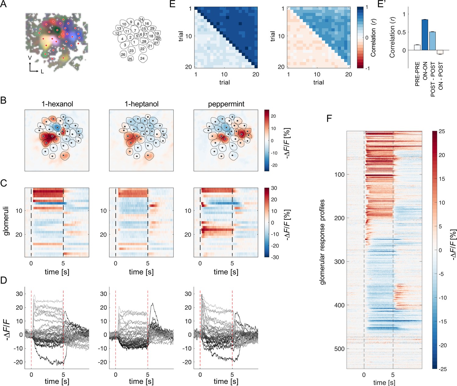
(A) For each AL, the odour response maps for the three stimuli were merged into an RGB image to highlight glomerular structures: 1-hexanol was set as the red channel, 1-heptanol as the green, and peppermint as the blue. Glomeruli were hand-labelled for time-series extraction. V, ventral; L, lateral. (B) Exemplary AL odorant responses during olfactory stimulation with three odorants. Colour bar indicates the relative change of activity during olfactory stimulation with respect to the pre-stimulus baseline. Circular areas indicate identified glomeruli according to (A). (C, D) Temporal profiles of the glomerular regions identified in (A) for the three odorants. Each line in (C), labelled from 1 to 28, refers to the glomerular ID in (A). Temporal profiles represent the average activity of 20 stimulations. Dashed lines in (C, D) limit the begin and the end of the olfactory stimulation. (E, E') Pearson’s correlations between pairs of glomerular response vectors across repetitions. (left) The upper right part of the matrix shows correlation scores among glomerular activity during olfactory stimulation (t=1–5 s after odorant onset, ON vs ON) across trials; the bottom left part shows correlation scores among glomerular activity before stimulation (t = –1–0 s, PRE vs PRE) across trials. (right) The upper right part of the matrix shows correlation scores among glomerular activity after olfactory stimulation (t=1–4 s after odorant offset, POST vs POST) across trials; the bottom left part shows correlation scores among glomerular activity during and after stimulation (ON vs POST) across trials. (E') Mean (± s.e.m.) across-trial correlation of the four combinations presented in the matrices in (E). (F) All glomerular responses from eight ALs to three odorants were pooled together to provide an overview of the complexity of response profiles (n=546).
Figure 1—figure supplement 1
Sample of glomerular response profile dynamics across trials.
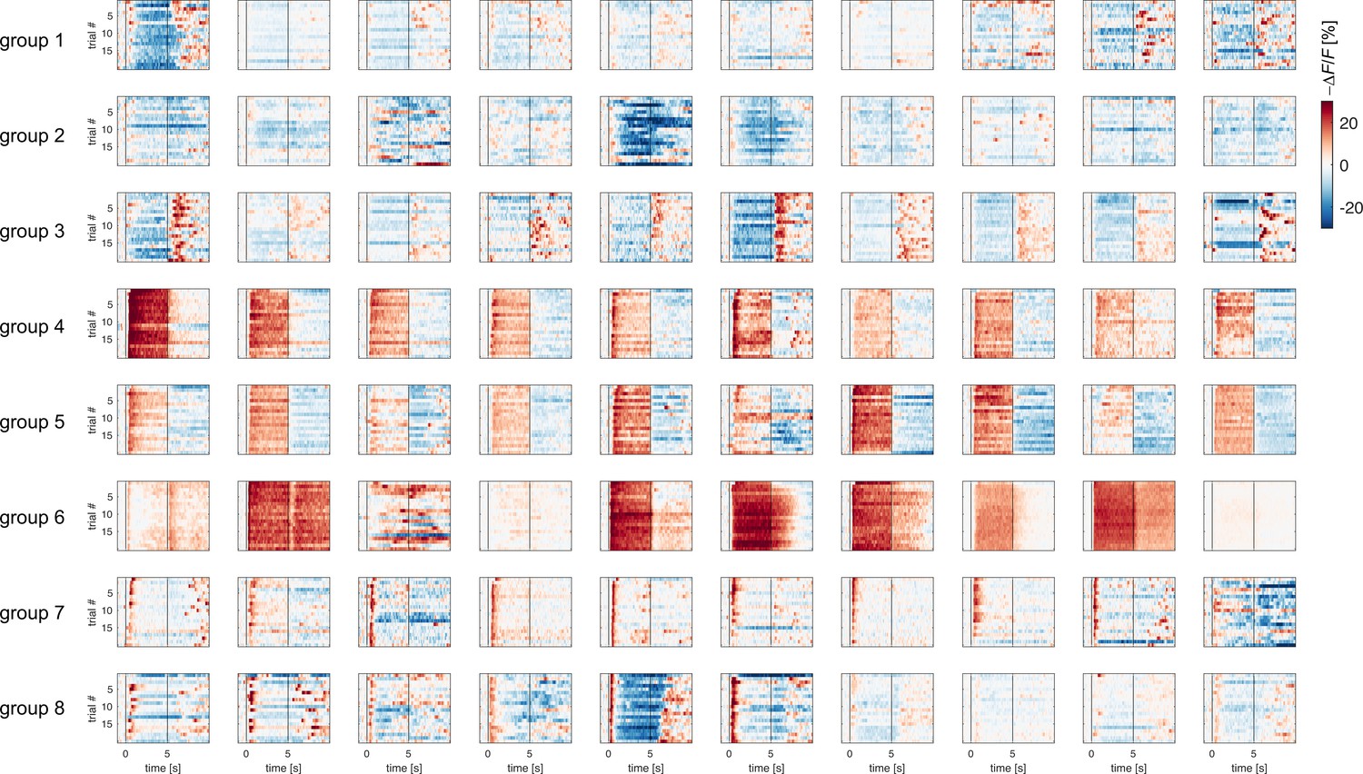
Each subplot displays the response profile across 20 repetitions of the same odorant for one glomerulus. For exemplificatory purpose, a subset of 10 glomerular response profiles from response groups 1–8 (80 out of 464) is shown. Vertical lines indicate stimulus onset and offset.
Figure 2 with 1 supplement
Clustering of projection neurons' response profiles.
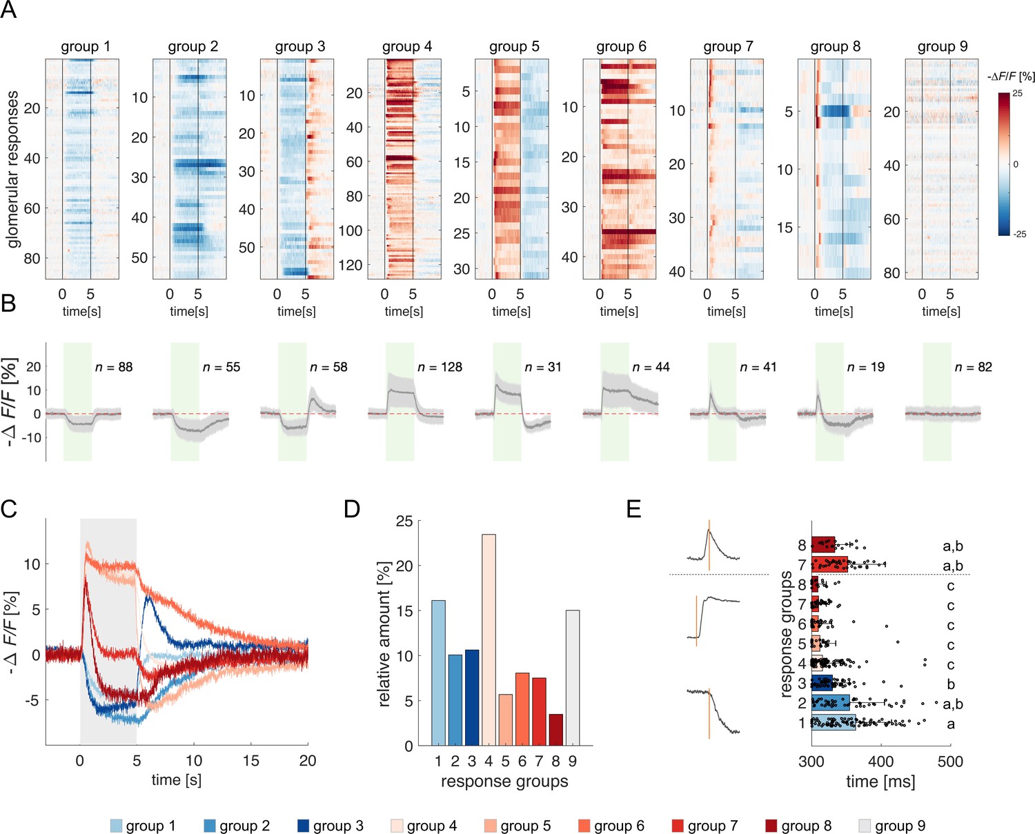
(A) All glomerular responses were clustered with supervision according to their activity (excitatory, inhibitory, non-responsive) during and after stimulus arrival. (B) Mean ± s.e.m. of all curves of the relative groups in (A). The green patch indicates the stimulus delivery interval. (C) Average curves of all response groups from (B) are superimposed. The grey patch indicates the stimulus delivery interval. (D) Relative amount of all response categories. (E) Latency of glomerular responses for excitatory and inhibitory profiles (groups 1–8). For groups 7 and 8, the latency of short excitatory response’s termination was calculated. Letters refer to significative groups after Kruskal-Wallis statistical test and Tukey-Kramer correction. On the left side, exemplary traces of phasic and tonic excitatory responses and an inhibitory response are shown. The orange line indicates the latency of response onset or termination.
Figure 2—figure supplement 1
Odorant response profiles for each bee and stimulus.
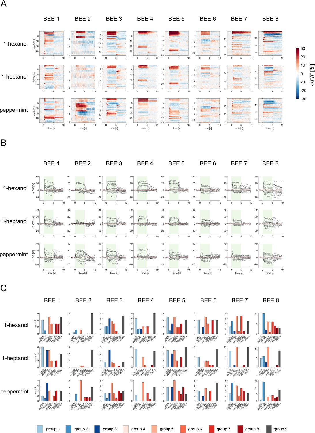
(A) Responses from eight bees to three odorants. Each raster plot shows the average response profile of 20 stimulus repetitions. Stimulation occurs between 0 and 5 s. (B) Glomerular response profiles of all detected glomeruli (as in A) are shown as time traces. Green bars indicate stimulus intervals. Each trace is the mean of 20 stimulus repetitions. (C) Occurrence of the varied response profiles for each bee/odorant condition.
Figure 3
A simple neural network model for olfactory coding and learning.
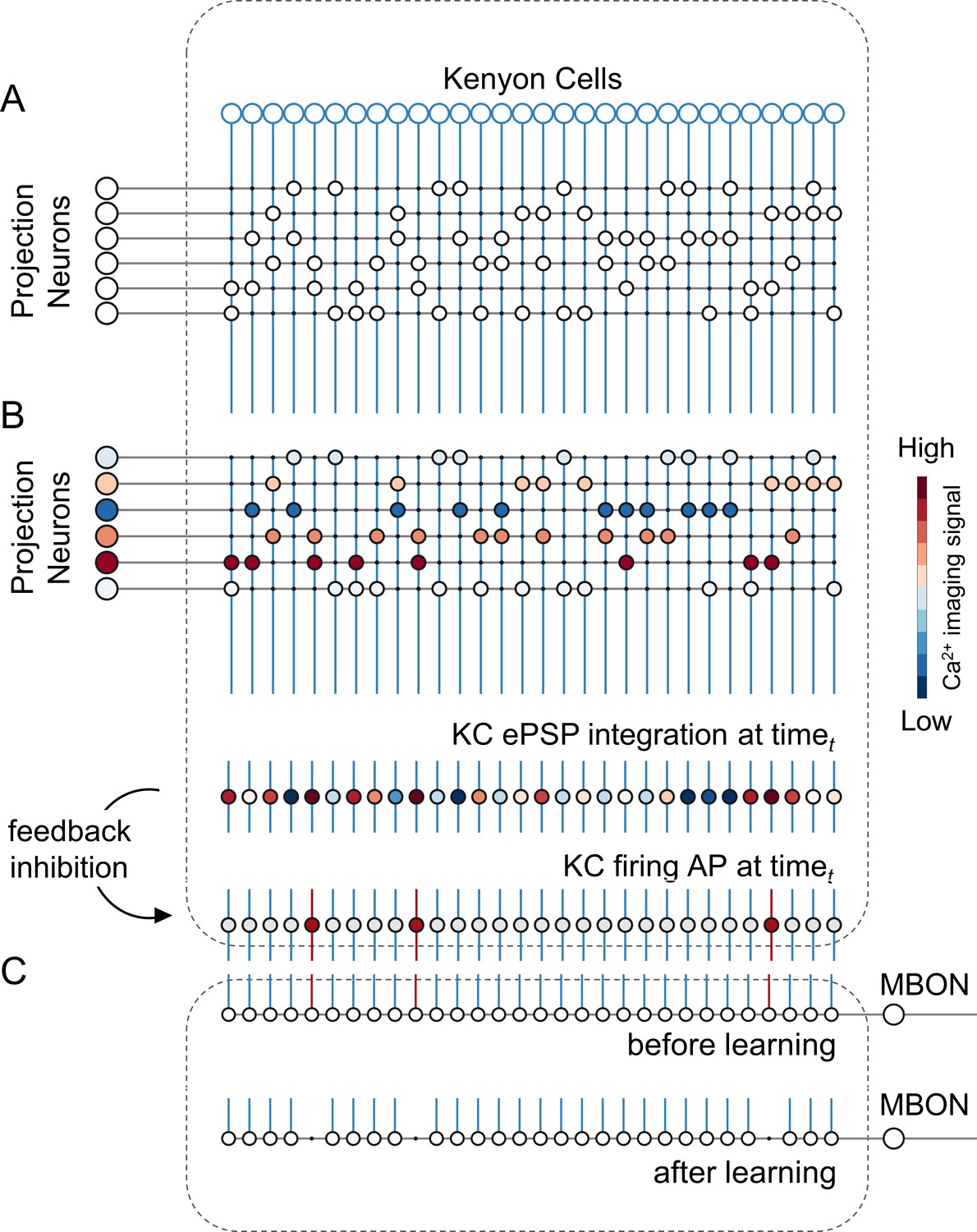
(A) The synaptic connectivity between AL PNs and KCs is built as a pseudorandom logic matrix where each column represents KC dendritic arborisation and each row PN axon terminals. Each KC receives synaptic contact – here represented as a white circle – from 30% of the PN population. (B) For each timepoint t of a calcium imaging recording, the measured activity level for each glomerulus (represented by a PN in the model) is projected onto all its synaptic connections with the KC population. Each KC, that is each column in the scheme, integrates all excitatory post-synaptic potentials. Finally, recurrent inhibitory feedback is simulated by imposing that only the 10% most active KCs will generate an action potential (AP) (red cells), while all others remain silent (grey cells). (C) A single appetitive MBON receiving input from all KCs was modelled. Based on a synaptic plasticity threshold parameter, all synapses from KCs to MBON that are activated with a frequency greater than allowed by the defined threshold during the learning window will be switched off. This phenomenon results in a decrease AP probability in the modelled MBON upon stimulation with the learned stimulus. Abbreviations: action potential, AP; antennal lobe, AL; excitatory post-synaptic potential, ePSP; Kenyon cells, KC; mushroom body, MB; mushroom body output neuron, MBON; projection neurons, PN.
Figure 4 with 2 supplements

Olfactory representation in modelled Kenyon cells (KCs).
(A) The first row displays the recorded PN responses of one honey bee to three odorants. The second row shows the transformation of the PN activity operated by the model to simulate the activity of 1000 KCs. In each plot, KCs are ordered for response strength during the onset and offset to better visualise activity clusters. (B) Turnover rate of recruited KCs across adjacent time points. Light blue traces refer to individual bees (mean of 10 MB simulations). Thick, dark blue traces indicate average curves across bees. (C) Cumulative recruitment of KC shows two main recruitment events at stimulus onset and offset. To observe odorant-related KC recruitment dynamics, the cumulative sum was initiated at stimulus onset. Light blue traces refer to individual bees (mean of 10 MB simulations). Thick, dark blue traces indicate average curves across bees. (D, E) Correlation matrix among time points of measured PN activity (C) and simulated KC activity (E). Mean responses to the three odorants were concatenated to allow observing within and across odorant correlations. (F) PCA of odorants' trajectories in the measured PN space (top) and in the modelled KC space (bottom) for four exemplary bees. Trajectories comprise a 10 s interval, ranging from odour onset (t=0 s, light) to 5 s after offset (t=10 s, dark). (G) The raster plot shows a set of 100 artificially combined glomerular responses (top), each simulating the neural representation of 100 similar odorants in the PN space. A second raster plot (middle) shows the representation of the same odorants in the modelled KC space. Note that odorant representation was considered as the mean activity of PN (or KC) during stimulus arrival (0.5–5 s). The histogram shows the distributions of between-odorant correlations computed among all pairs of odour vectors in the PN and KC space. A significant difference between the two distributions was tested with a Student’s t test (p 0, n=4774).
Figure 4—figure supplement 1
Odorant-specific activity lasts longer in the Kenyon cells space.
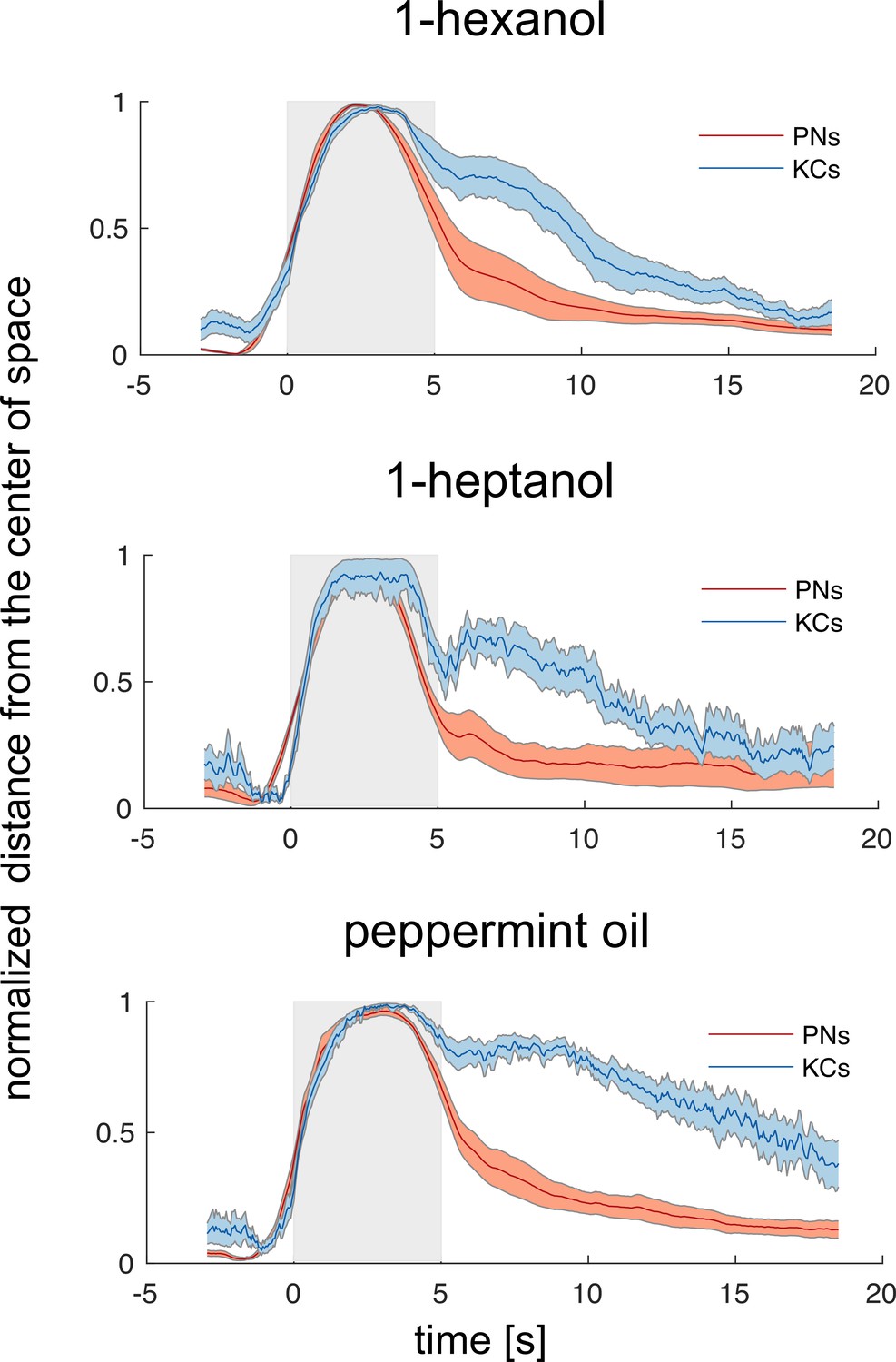
Time traces of the normalised Euclidean distance from the centre of coordinates (where the centre of coordinates was set to 0 and the maximum distance from it was set to 1) in the PN and KC space for the three odorants. This transformation allowed performing a direct comparison between the temporal dynamics of the representations of one odorant in the PN and KC space. Discriminability – that is, distance from 0 – peaks during olfactory stimulation but is maintained longer in the KC space. Notably, such a long-lasting odorant-specific signature is not achieved by maintaining onset-recruited neurons activity for a longer period of time but by recruiting two pools of KCs (both odorant-specific): one for the ON phase and one during the OFF phase (see also Figure 4). Grey patches indicate stimulation windows. Traces represent mean ± s.e.m. of eight animals (PN data, red) and relative MB simulations (KC data, blue).
Figure 4—figure supplement 2
Dependence of Simulated MBON Activity on Synaptic Plasticity Threshold.
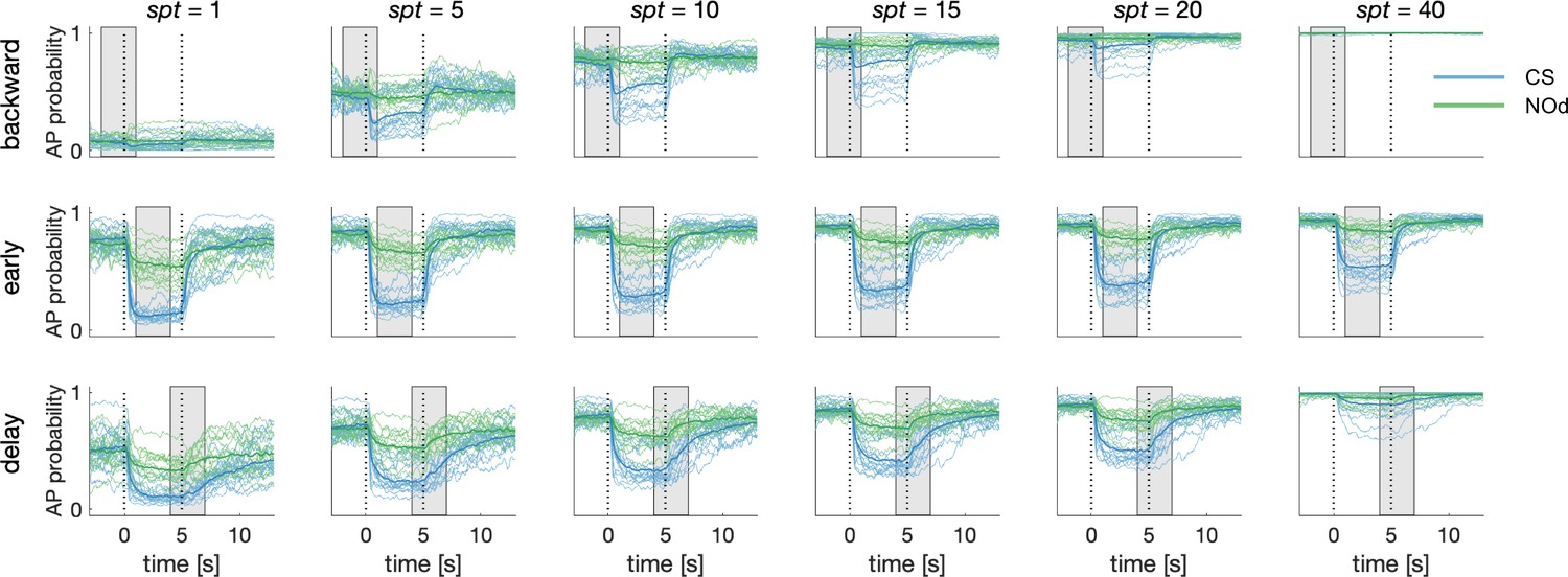
Synaptic plasticity threshold (spt) dictates how many times a KC-to-MBON synapse has to be recruited during the learning window before being switched off. The influence of spt on MBON learning was tested for all CS/US protocols. The extreme values of the parameters (spt = 1 and 40) indicate that a certain synapse should be recruited only once or 40 times before being turned off (note that to be activated 40 times in a 3 s learning window and with 20 Hz sampling rate, a synapse should fire for two entire seconds). With the exceptions of the extreme parameters, the MBON AP probability upon CS and NOd presentation is only weakly affected by spt value. Notably, a small spt results in higher generalised learning, while a large spt requires a stable KC signal for synapses to be modulated and produces weaker learning scores.
Figure 5
Modelled mushroom body output neurons can predict behavior.
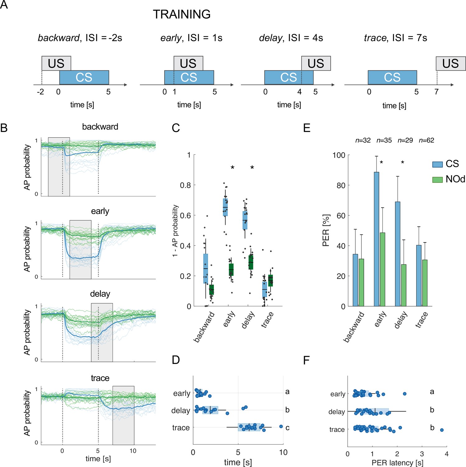
(A) Four experimental protocols differing for CS/US inter stimulus interval (ISI) were used for training the model (B–D) and for behavioural measurements of the proboscis extension reflex (PER) conditioning (E, F). Trained simulated MBONs, as well as conditioned honey bees were tested against the conditioned stimulus (CS, blue) and a novel odorant (NOd, green). (B) Time course of action potential (AP) probability of a trained MBON upon stimulation with the CS (blue) or with the novel odorant (green). Olfactory learning was modelled according to backward, early, delay, and trace conditioning protocols. Glomerular responses for eight bees to 1-hexanol and peppermint oil were used alternatively as CS and NOd. Data for responses to CS and NOd were pooled together (n=16 traces for each protocol). Thick trace: average AP probability profile; dotted vertical lines: stimulus onset/offset; grey bar: modelled learning window. (C) Distribution of the mean values of traces in (B) during CS and NOd stimulation. Because appetitive learning produces a decrease in MBON firing rate, the complementary value of the probability fraction provides a proxy for a learned appetitive response (Kruskal-Wallis statistical test: pbackward = 0.0545; pearly = 1.42*10–6; pdelay = 1.04*10–5; ptrace = 0.0595; n=16). (D) Latency of 90% of minimal MBON activity in response to the CS for early and delay conditioning protocols (Wilcoxon test early vs delay, p=0.0015; delay vs trace, p=0.0005. Letters indicate statistical groups according to the Wilcoxon test. Barlett’s test for variance difference early vs delay, p=1.73*10–6; delay vs trace, p=0.1808; early vs trace p=1.29*10–8). (E) Memory retention test of honey bees 1 hr after absolute conditioning. Bars indicate the percentage of individuals showing proboscis extension reflex (PER) when presented with the conditioned (blue) or the novel odorant (green). Error bars indicate 95% confidence intervals. (Responses to the CS/NOd were compared with a McNemar test for binomial distribution; pearly = 0.003, pdelay = 0.004). (F) Latency of the PER to the conditioned stimulus at the 1 hr memory retention test (Kruskal-Wallis statistical test: early vs delay, p=0.036; early vs trace. p=0.041; delay vs trace, p=0.992. Letters indicate statistical groups according to the Kruskal-Wallis test. Barlett’s test for variance difference across protocols: early vs delay, p=5.19*10–6; early vs trace. p=0.020; delay vs trace, p=0.007; nearly = 26; ndelay = 20; ntrace = 31).
Figure 6
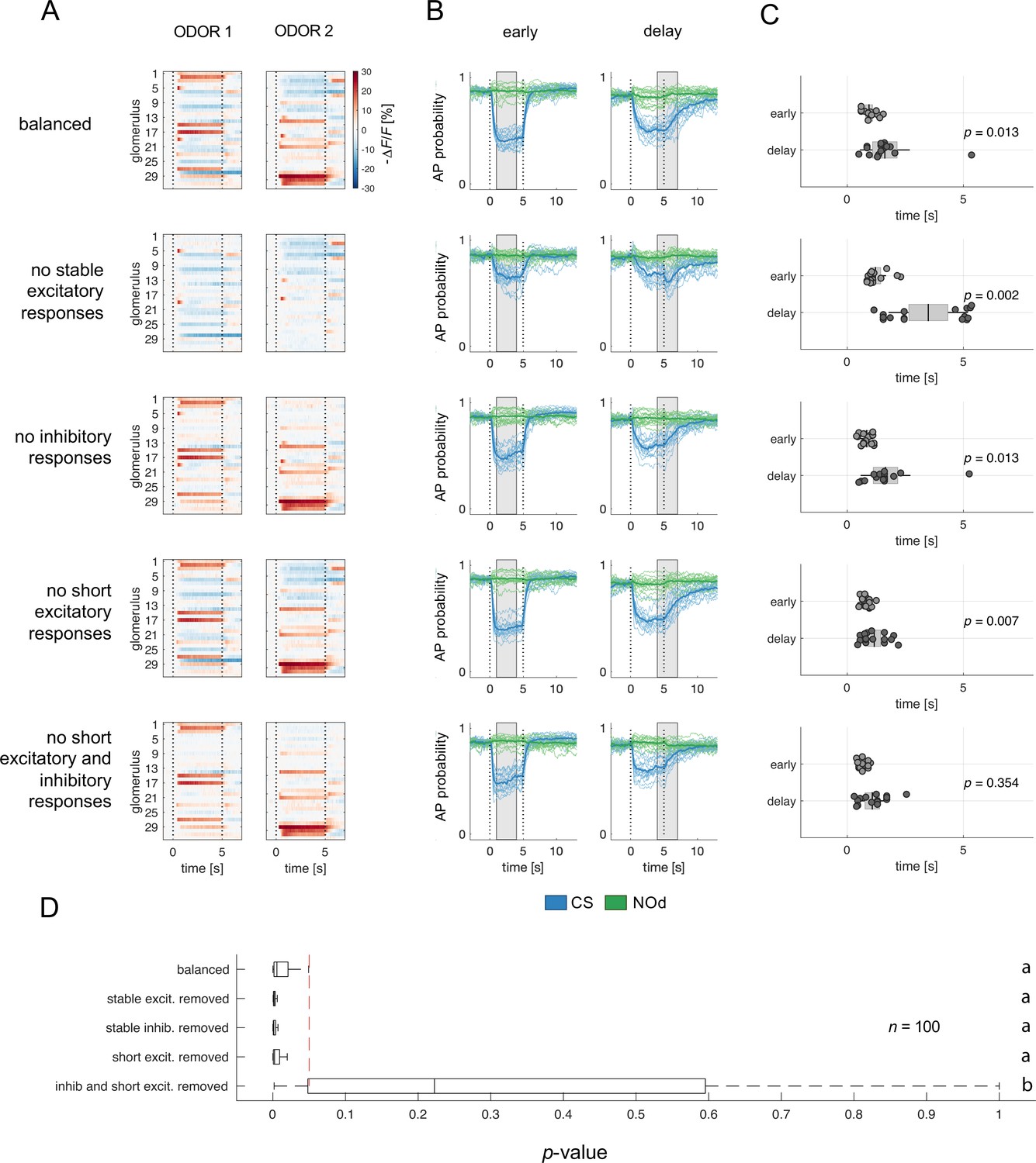
Relative contribution of glomerular response types to MBON response latency.
(A) Two instances of odorant responses generated by artificially combining 32 glomerular response profiles from all response groups from Figure 2 (first row). Response profiles were manipulated eliminating stable excitatory responses (second row), inhibitory responses (third row), short excitatory responses (fourth row), and short excitatory and inhibitory responses together (last row). Dotted lines indicate stimulus onset and offset. (B) Time course of action potential (AP) probability of a trained MBON upon stimulation with the conditioned stimulus (CS, blue) or with the novel odorant (NOd, green). Olfactory learning was modelled according to early and delay conditioning protocols and with the balanced (first row) and modified simulated odorants (second to last row). Conditioned stimulus and novel odorant are in blue and green, respectively (n=16). Thick trace: average AP probability profile; dotted vertical lines: stimulus onset/offset; grey bar: modelled learning window. (C) Latency of 90% of minimal MBON activity in response to the CS for early and delay conditioning protocols (Wilcoxon signed rank test early vs delay; n=16). (D) Distribution of Wilcoxon signed rank test p-values of 100 simulations of (C). The red dashed line indicates a significance level of 0.05; letters indicate significance groups.
Additional files
Download links
A two-part list of links to download the article, or parts of the article, in various formats.
Downloads (link to download the article as PDF)
Open citations (links to open the citations from this article in various online reference manager services)
Cite this article (links to download the citations from this article in formats compatible with various reference manager tools)
Analysis of fast calcium dynamics of honey bee olfactory coding
eLife 13:RP93789.
https://doi.org/10.7554/eLife.93789.3


