Intrinsic dynamics of randomly clustered networks generate place fields and preplay of novel environments
Figures
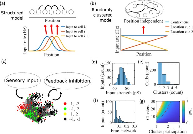
Illustration of the randomly clustered model.
(a) Schematic diagram of prior replay models that rely on preexisting environment-specific structure, wherein each cell receives uniquely tuned Gaussian-shaped feed-forward inputs to define the place fields, and cells with nearby place fields are recurrently connected. Pairs of cells with closest place fields are connected most strongly (thicker arrows). (b) Schematic diagram of our model, where neurons are randomly placed into clusters and all neurons receive the same spatial and contextual information but with random, cluster-dependent input strengths. (c) Example representation of the network (8 clusters, mean cluster participation per cell of 1.5). Excitatory cells (each symbol) are recurrently connected with each other and with inhibitory cells (‘Feedback inhibition’, individual inhibitory cells not shown) and receive feed forward input (‘Sensory input’). Symbol color indicates neurons’ membership in clusters 1 and 2, with ~meaning not in the cluster. Symbol size scales with the number of clusters a neuron is in. Lines show connections between neurons that are in cluster 2. Symbol positions are plotted based on a t-distributed stochastic neighbor embedding (t-SNE) of the connection matrix, which reveals the randomly overlapping clusters. (d-f) Histograms based on the network in (c) of: (d) the distribution of input strengths; (e) the number of clusters that each neuron is a member of; and (f) the fraction of the excitatory cells to which each excitatory cell connects. (g) The Small-World Index (SWI) of the excitatory connections varies with the number of clusters and the mean number of clusters of which each neuron is a member (“cluster participation”). The median value of the SWI from 10 networks at each parameter point is plotted. The red dashed line shows a contour line where SWI = 0.4. Regions in white are not possible due to either cluster participation exceeding the number of clusters (lower right) or cells not being able to connect to enough other cells to reach the target global connectivity (upper left).
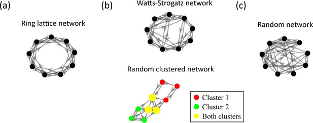
Comparison of the randomly clustered network and the canonical Watts-Strogatz small-world network.
(a) A small ring-lattice network. (b) Example small-world networks. Top, a Watts-Strogatz network with re-wiring parameter . Bottom, a randomly clustered network with two clusters and a cluster participation of 1.25. (c) Example randomly connected network.
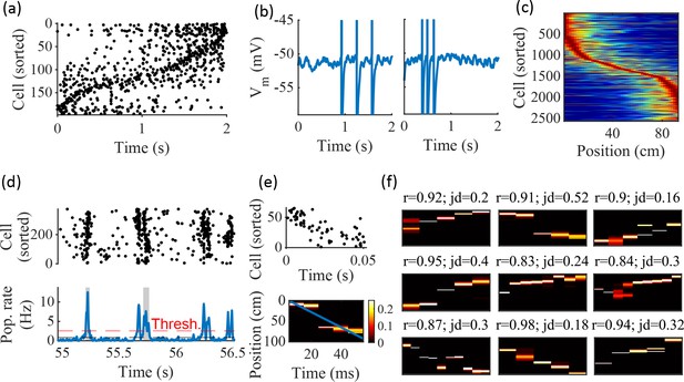
Spatially correlated reactivations in networks without environment-specific connectivity or plasticity.
(a–f) Example activity from the fiducial parameter set (15 clusters, mean cluster participation of 1.25). (a) Example raster plot from one place-field trial. Cells sorted by trial peak. (b) Example membrane traces from two of the cells in (a). (c) Place fields from 10 different networks generated from the same parameter set, sorted by peak location and normalized by peak rate. (d) Example raster plot (top) and population firing rate (bottom; blue line) showing preplay in a simulation of sleep. Horizontal dashed black line is the mean population rate across the simulation. Horizontal dashed red line is the threshold for detecting a population-burst event (PBE). PBEs that exceeded the threshold for at least 50 ms and had at least five participating cells were included in the preplay decoding analysis. Grey bars highlight detected events. (e) Example preplay event (Top, raster plot. Bottom, Bayesian decoding of position). Event corresponds to the center event in (d). Raster includes only participating cells. The blue line shows the weighted correlation of decoded position across time. (f) Nine example decoded events from the same networks in (c). The width of each time bin is 10 ms. The height spans the track length. Same color scale as in (e). r is each event’s absolute weighted correlation. jd is the maximum normalized jump in peak position probability between adjacent time bins. The same event in (e) is shown with its corresponding statistics in the center of the top row. Preplay statistics calculated as in Farooq et al., 2019.
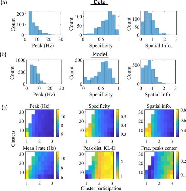
The model produces place fields with similar properties to hippocampal place fields.
(a) Place field statistics for hippocampal place fields recorded in rats upon their first exposure to a W-track (Shin et al., 2019).
Left, place-field peak rate (Hz). Center, place-field specificity (fraction of track). Right, place-field spatial information (bits/spike). (b) Same as (a) but for place fields from a set of 10 simulated networks at one parameter point (15 clusters and mean cluster participation of 1.25). (c) Network parameter dependence of place-field statistics. For each parameter point, the color indicates the mean over all place fields from all networks. Top row: mean statistics corresponding to the same measures of place fields used in panels (a, b). Bottom left: mean firing rate of the inhibitory cells. Bottom center: the KL-divergence of the distribution of place-field peaks relative to a uniform spatial distribution. Bottom right: fraction of place-field peaks peaked in the central third of the track.
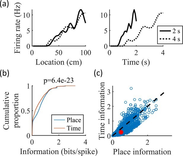
The simulated cells have greater place information than time information.
(a) Place fields (left) and time fields (right) for an example cell calculated from simulated trajectories that took 2 s (solid line) or 4 s (dotted line) to traverse the track. (b) CDFs of the information content of the place fields (‘Place’) and time fields (‘Time’) of all cells. The spatial information is significantly greater than the temporal information (KS-test, p=6.4e-23). (c) Scatter plot of the data in (b), with the median values marked in red.
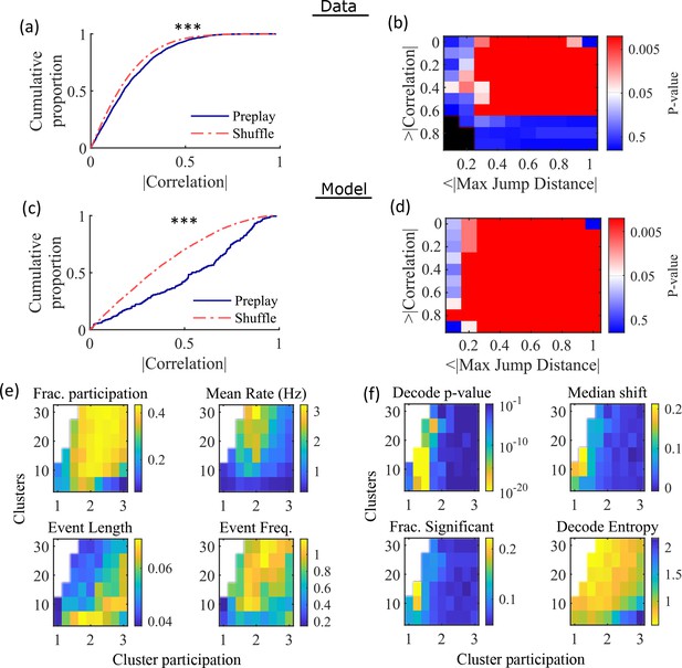
Preplay depends on modest cluster overlap.
(a, c) The cumulative distribution function (CDF) of the absolute weighted correlations for actual events (blue line) versus shuffled events (red dashed line) of experimental data from Shin et al., 2019 (a; KS-test, p=2 × 10–12, KS-statistic=0.078) and simulated data (c; KS-test, p=3 × 10–16, KS-statistic=0.29) reveal results similar to those in Figure 1h of Farooq et al., 2019. *** p<0.001. (b, d) p-value grids (p-value indicated logarithmically by color) showing that the actual decoded events are higher quality sequences than shuffles across a wide range of quality thresholds for both experimental data from Shin et al., 2019 (b) and simulated data (d). For each point on the grid, the fraction of events that exceed the absolute weighted correlation threshold (y-axis) and don’t exceed the maximum jump distance (x-axis) is calculated, and the significance of this fraction is determined by comparison against a distribution of corresponding fractions from shuffled events. Black squares indicate criteria that were not met by any events (either shuffled or actual). The panel is equivalent to Figure 1e of Farooq et al., 2019. (e) Network parameter dependence of several statistics quantifying the population-burst events. Top left, fraction of excitatory cells firing per event. Top right, mean excitatory cell firing rate (Hz). Bottom left, mean event duration (s). Bottom right, mean event frequency (Hz). Each point is the mean of data combined across all population-burst events of all networks at each parameter point. Data from the same simulations as Figure 3. (f) Network parameter dependence of several statistics quantifying the Bayesian decoding. Top left, p-value of the absolute weighted correlations (from a KS-test as calculated in (c)). Top right, the shift in the median absolute weighted correlation of actual events relative to shuffle events. Bottom left, the fraction of events with significant absolute weighted correlations relative to the distribution of absolute weighted correlations from time bin shuffles of the event. Bottom right, the mean entropy of the position probability of all time bins in decoded trajectories.
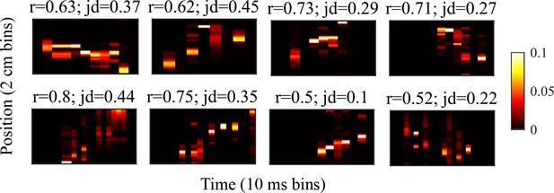
Example preplay events from the Shin et al., 2019 data.
Example preplay events. Same as Figure 2f but for events from the hipopcampal data from Shin et al., 2019. The height of each plot spans the length of the trajectory used for decoding, divided into 2 cm spatial bins. The width of each plot spans the duration of the detected event, divided into 10 ms time bins. Probability is show in color.

Significant preplay can typically be identified with as few as 50 cells.
(a–c) Results from performing the same Bayesian decoding on the same simulated population burst events (PBEs) in Figure 4c but using only random subsets of the excitatory cells for performing the decoding analysis. Each circle is the result of an analysis performed on one random subset of the cells. 25 random subsets were analyzed for each analyzed cell count. The subset sizes are logarithmically spaced. Black lines show the median value. The variability at N=375 is due to the variation in the randomness of the time-bin shuffles. (a) Number of events meeting the inclusion criterion for decoding analysis. (b) p-value of the KS-test comparing actual vs shuffled event absolute weighted correlations. A majority of the random subsets of 50 cells (17 out of 25) produce preplay p-values below 0.05. (c) Shift in the median absolute weighted correlation of actual events relative to shuffled events.
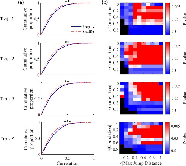
Preplay statistics by trajectory for Shin et al., 2019 data.
(a) Same as Figure 4a but separated by results from decoding by each of the 4 trajectories of the W-track individually (trajectory 1, center arm to right arm; trajectory 2, right arm to center arm; trajectory 3, center arm to left arm; trajectory 4, left arm to center arm). KS-test for each trajectory: trajectory 1, p=0.0030; trajectory 2, p=0.0028; trajectory 3, p=0.0027; trajectory 4, p=5.461 × 10⁻⁵. ** p<0.01, *** p<0.001. (b) Same as Figure 4b but separated by results from decoding by each of the four trajectories individually.
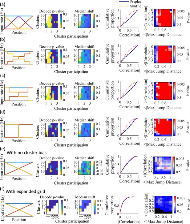
Additional simulations support the consistency and robustness of the model to variations in spatial input forms.
Each row corresponds to a different parameter grid simulation, with statistics calculated as in the corresponding panel from Figure 4. (a) Preplay statistics are similar to the main simulation results when a third linearly varying spatial cue is included in the inputs to the network (CDF KS-test, p=3.9e-13, KS-statistic=0.26). (b) Preplay statistics are similar to the main simulation results when a stepped input is used (CDF KS-test, p=2.5e-08, KS-statistic=0.20). The stepped input is less spatially informative since stretches of adjacent locations on the track have identical spatial input. (c) Same as (b), but with three step increments (CDF KS-test, p=6.2e-13, KS-statistic=0.26). (d) Same as (c), but with a single step increment (CDF KS-test, p=4.9e-13, KS-statistic=0.26). With this input the fiducial parameter set still shows significant preplay (right two columns), but most of the parameter grid loses significant preplay. (e) When the bias in cluster spatial input location is removed preplay is no longer significant (CDF KS-test, p=0.34, KS-statistic=0.063). (f) A parameter grid that shows greater values of cluster participation do not have significant preplay. Values along the diagonal where clusters equals cluster participation are equivalent to a random cluster-less network. Example parameter point is at clusters = 5 and cluster participation = 5 (CDF KS-test, p=0.99, KS-statistic=0.02).
Coherent spiking within clusters supports preplay.
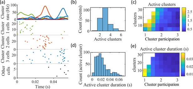
(a) Example event. Top, spike rates averaged across neurons of individual clusters: Each firing rate curve is the smoothed mean firing rate across the population of cells belonging to each cluster. We defined clusters as ‘active’ if at any point their rates exceed twice that of any other cluster. Three clusters meet the criterion of being active (green, then red, then blue). Bottom, raster plots: Cells belonging to each of the active clusters are plotted separately in the respective colors. Cells in multiple clusters contribute to multiple population curves, and cells in multiple active clusters appear in multiple rows of the raster plot. Cells that participate but are not in any active clusters are labeled ‘Other cells’ and plotted in black. Only active cells are plotted. (b) For the fiducial parameter set (15 clusters, mean cluster participation of 1.25), the distribution over events of the number of active clusters per event. (c) The mean number of active clusters per event as a function of the network parameters. Same data as that used for the parameter grids in earlier figures. (d) For the fiducial parameter set (15 clusters, mean cluster participation of 1.25), the distribution of durations of active clusters for all active cluster periods across all events. The active duration was defined as the duration for which an active cluster remained the most-active cluster. (e) The mean active cluster duration as a function of the network parameters.

Relationship between cluster activation and preplay.
(a) Out of all events from the fiducial parameter set simulations where three unique clusters were active, the fraction of those events with sequences that match the order of cluster biases on the track (red line) is consistent with the values expected by randomly sampling clusters (blue). (b) Z-scored absolute weighted preplay correlation is negatively correlated with the number of active clusters (Spearman’s rank correlation).
Preplay is abolished when events are decoded with shuffled cell identities but is preserved if cell identities are shuffled only within clusters.
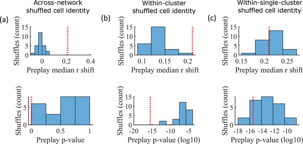
We decoded the population burst events from the fiducial parameter set simulations after randomly shuffling cell identities in three different manners (a-c, 25 replicates for each condition) and compared the resulting preplay statistics to the unshuffled result (red line). (a) Randomly shuffling cell identities results in median preplay correlation shifts near zero (top, 100th percentile of shuffles), with p-values distributed approximately uniformly (bottom, 0th percentile of shuffles). (b) Randomly shuffling cell identities within clusters reduces the magnitude of the median preplay correlation shifts (top, 100th percentile of shuffles) but preserves the statistical significance of preplay (bottom, 0th percentile of shuffles). (c) Randomly shuffling cell identities within clusters for only cells that belong to a single cluster results in median preplay correlation shifts that are similar to the unshuffled result (top, 36th percentile of shuffles) and are all statistically significant (bottom, 12th percentile of shuffles).
Place cells’ mean event rank are correlated with their place field location when accounting for decode direction.
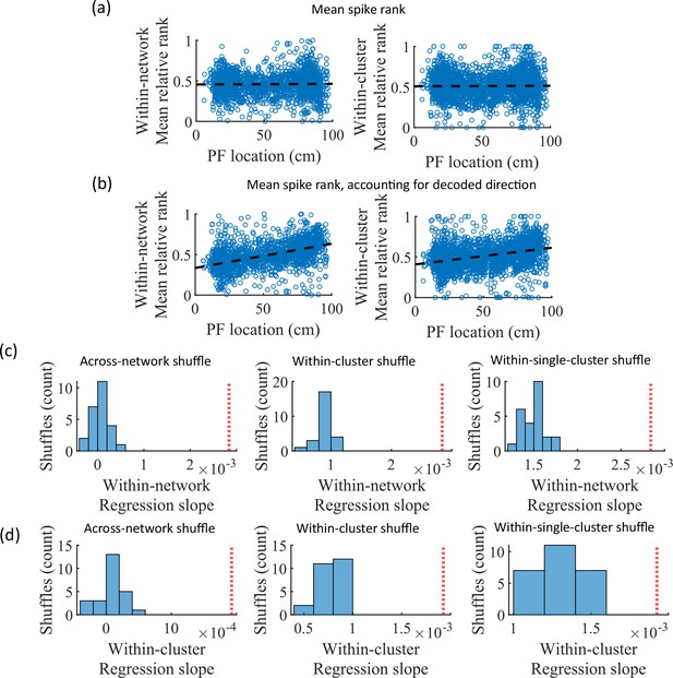
(a) Mean within-event relative spike rank of all place cells as a function of the location of their mean place field density on the track for networks at the fiducial parameter set. Left, mean relative rank with respect to all cells in each network. Right, mean relative rank with respect to only cells that share cluster membership. (b) Same as (a), but after accounting for the direction of each events’ decoded trajectory. If the decoded slope for a given event was negative, then the order of spiking in that event was reversed. (c, d) Comparison of the regression slopes from (b) to the distribution of slopes that results from applying the same analysis after shuffling cell identities as in Figure 6. (c) The within-network regression slope is significant relative to all three methods of shuffling cell identity. (d) Same as (c), but for the within-cluster regression slope.
The Small-World Index of networks correlates with preplay quality.
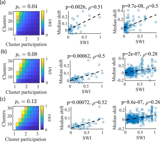
(a–c) Left column, the Small-World Index (SWI; plotted as color) is affected by the global E-to-E connection probability, . Red dotted line indicates a contour line of SWI = 0.4. This boundary shifts downward as increases. Center column, across parameter points in the network parameter grid, SWI correlates with an increase in the median absolute weighted correlation of decoded trajectories relative to shuffles (e.g. this corresponds in Figure 4c to the rightward shift of the CDF of measured absolute weighted correlations relative to the shuffle events). Each point is produced by analysis of all events across 10 networks from one parameter point in the grid on the left. Right column, same as the center column but each point is data from each of the 10 individual networks per parameter set. p-value and correlation, , are calculated from Spearman’s rank-order correlation test. Dashed line is the least-squares fit. (a) Data from a parameter grid where the E-to-E connection probability was decreased by 50% and the E-to-E connection strength was doubled from their fiducial values used in prior figures. (b) Data from the same parameter grid as Figures 3—5. (c) Data from a parameter grid where the E-to-E connection probability was increased by 50% and the E-to-E connection strength scaled by two-thirds from their fiducial values.
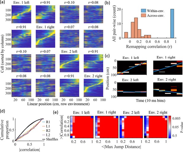
Trajectories decoded from population-burst events are significantly correlated with linear trajectories in arbitrary environments.
(a) Place fields from a single network with simulated runs in both directions of travel on a linear track in two different environments. Each column of panels is the set of place fields for the trajectory labeled on the diagonal. Each row of panels has cells sorted by the order of place-field peaks for the trajectory labeled on the diagonal. The r values are the correlations between the corresponding remapped trajectory with its comparison on the diagonal. Note that correlations mirrored across the diagonal are equal because they correspond only to a change in the labels of the dimensions of the population rate vectors, which does not affect the vector correlation. (b) Distribution of the place-field map correlations across trajectories from both directions of travel on a linear track in two environments for 10 networks. Blue is the distribution of correlations for all left vs right place-field maps from the same environment. Red is the correlations from all pair-wise comparisons of trajectories from different environments. (c) An example event with a statistically significant trajectory when decoded with place fields from Env. 1 left (absolute correlation at the 99th percentile of time-bin shuffles) but not when decoded with place fields of the other trajectories (78th, 45th, and 63rd percentiles for Env. 1 right, Env. 2 left, and Env. 2 right, respectively). (d) An entire set of PBEs shows similar levels of absolute weighted correlations when decoded with different sets of place fields. In color are CDFs of absolute weighted correlations of decoded trajectories with leftward and rightward linear trajectories in each of the two environments (R1 and L1 are the rightward and leftward trajectories of environment one. R2 and L2 are the rightward and leftward trajectories of environment two). In black (all overlapping) are the corresponding absolute weighted correlations with each of the four trajectories arising from decoding of shuffled events. (e) The significance of linearity of decoded trajectories indicated by p-value in color (as in Figure 4b) from decoding the same PBEs with the four different environment place fields. Black squares indicate criteria that were not met by any events (either shuffled or actual). Env. 1 left is the same as that shown in Figure 4d.


