Mapping responses to focal injections of bicuculline in the lateral parafacial region identifies core regions for maximal generation of active expiration
- Department of Physiology, University of Alberta, Canada
- Neuroscience and Mental Health Institute, University of Alberta, Canada
- Department of Psychology, University of Alberta, Canada
- Department of Anesthesiology and Pain Medicine, University of Alberta, Canada
- Women and Children’s Health Research Institute, University of Alberta, Canada
Figures
Figure 1
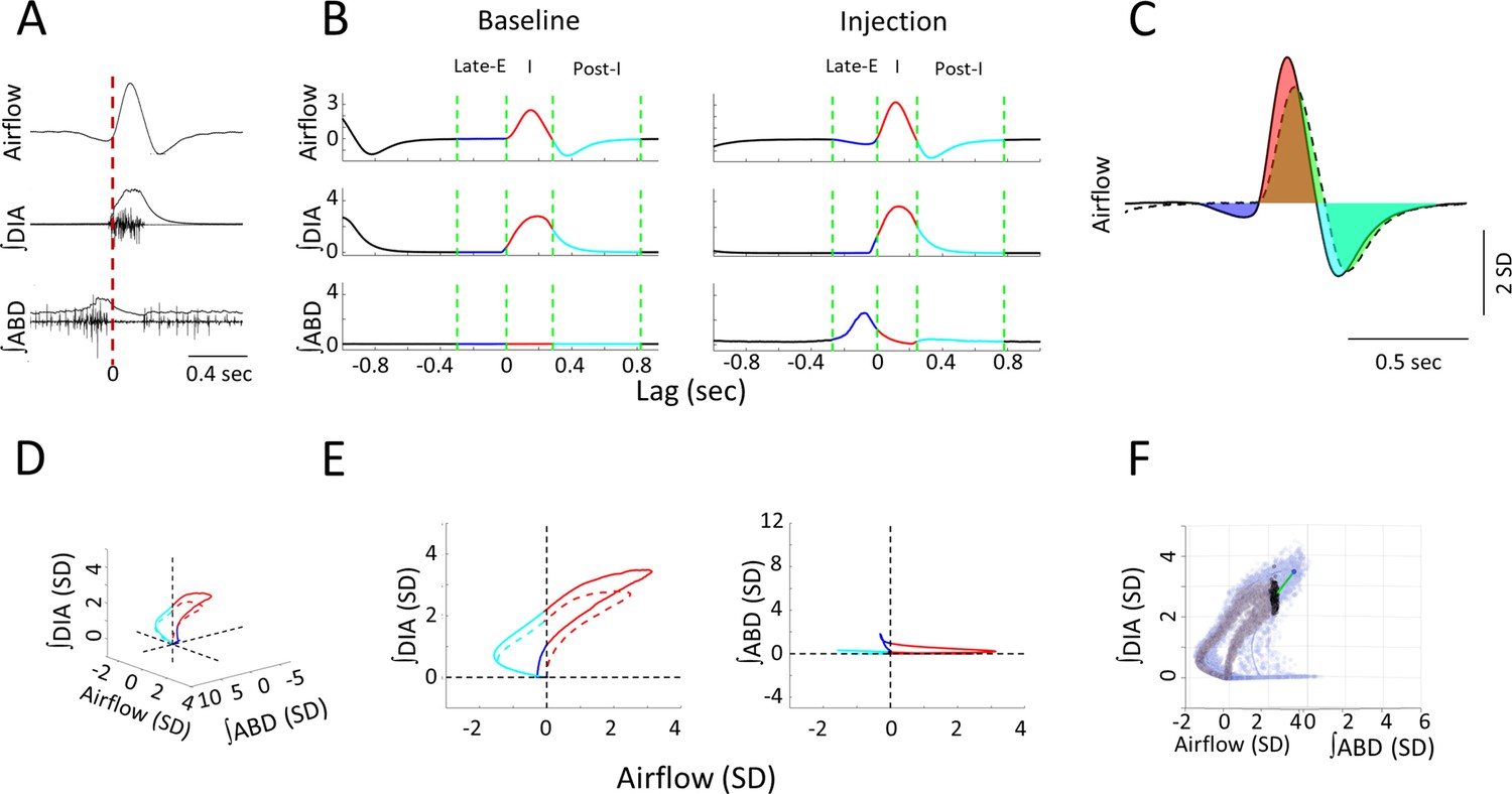
Measures used in quantifying respiratory responses to bicuculline injections.
(A) The time course of raw, and integrated electromyogram (EMG) signals relative to recorded airflow during a sample breath. Vertical red line indicates the onset of inspiration as defined by positive airflow. (B) Respiratory phases within a mean-cycle computed during baseline and post-injection for each recorded signal. Green lines mark the boundaries of each phase of the respiratory cycle, including the late-expiratory (late-E) (blue), inspiratory (red), and post-inspiratory (post-I) (cyan) phases. (C) Sample calculation of normalized area under the curve. Area under the baseline mean-cycle (dashed line, area in green) in each phase is subtracted from the corresponding colored area under the response mean-cycle (solid line, late-E: blue, inspiration: red, post-I: cyan) to give a measure of how inspiratory airflow has changed relative to baseline. (D) 3D representation of a representative baseline (dashed line) and response (solid line) mean-cycle. Each timepoint is a dot in 3D space defined by its airflow, ∫DIA EMG, and ∫ABD EMG measurements. Colors indicate respiratory sub-periods as in B. Dashed lines indicate the origin for each measure. (E) 2D projection of the mean-cycle in D. As per the colors in B, points on the left-hand side indicate expiration, points on the right-hand side indicate inspiration. (F) Sample calculation of Euclidean and Mahalanobis distance measures for representative mean-cycles during the baseline (gray) and response (orange). PinkGreen line indicates the Euclidean distance between the response and baseline at a single timepoint. Black indicates the distribution of baseline values at the same timepoint used to calculate the Mahalanobis distance. Mean-cycles have been rotated relative to D to expose these distances to the viewer. ABD, abdominal; DIA, diaphragm.
-
Figure 1—source data 1
Measures used in quantifying respiratory responses to bicuculline injections, dataset for Figure 1A–E.
- https://cdn.elifesciences.org/articles/94276/elife-94276-fig1-data1-v1.xlsx
-
Figure 1—source data 2
Measures used in quantifying respiratory responses to bicuculline injections, dataset for Figure 1F (abdominal electromyogram [EMG] dataset).
- https://cdn.elifesciences.org/articles/94276/elife-94276-fig1-data2-v1.zip
-
Figure 1—source data 3
Measures used in quantifying respiratory responses to bicuculline injections, dataset for Figure 1F (respiratory flow dataset).
- https://cdn.elifesciences.org/articles/94276/elife-94276-fig1-data3-v1.zip
-
Figure 1—source data 4
Measures used in quantifying respiratory responses to bicuculline injections, dataset for Figure 1F (diaphragm electromyogram [EMG] dataset).
- https://cdn.elifesciences.org/articles/94276/elife-94276-fig1-data4-v1.zip
Figure 2
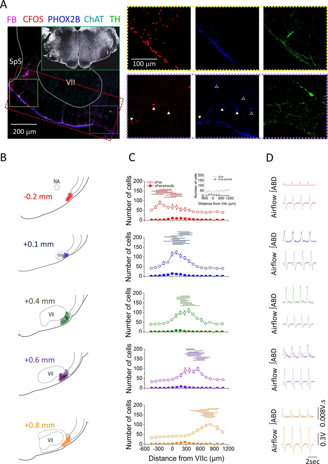
Location of bicuculline injections along the rostro-caudal axis of the ventral medulla.
(A) Representative confocal microscope images of immunohistochemistry performed at the injection sites. Red: cFos, cyan: ChAT, blue: PHOX2B, green: TH, magenta: fluorobeads. Inset shows bilateral injection sites at low magnification. Red rectangle is a representative example of the area used for cell counting. Yellow and purple squares are the areas represented on the right panel of A, notice the abundance of CFOS+ cells on the lateral area near the injection site (yellow square) compared to the fewer CFOS+ cells in the medial area (purple square). Closed white triangles are pointing out examples of CFOS-PHOXB+ cells, whereas open white triangles are pointing out examples of PHOX2B+ cells that were CFOS-negative. Magnification is the same for all images in the right panels of A. (B) Schematic representation of the core of the injection sites and the group attribution, according to proximity of injection sites among experimental rats (–0.2 mm, n=5; +0.1 mm, n=7; +0.4 mm, n=5; +0.6 mm, n=6; +0.8 mm, n=5). (C) Cell counting color coded according to the groups defined in B (CTRL, n=7; –0.2 mm, n=5; +0.1 mm, n=7; +0.4 mm, n=5; +0.6 mm, n=6; +0.8 mm, n=5). Data points represent the mean ± SEM of cells counted per hemisection at rostro-caudal locations ranging from –0.5 mm to +1.0 mm from VIIc. Open circles: CFOS+ cells; closed squares: CFOS/PHOX2B+ cells. Inset in group –0.2 mm is the cell count obtained for the CTRL group. Horizontal lines above the cell count graphs represent the rostro-caudal extension in which fluorobeads were observed for each injection site. (D) Representative examples of ∫ABD EMG and raw airflow traces obtained after injection of bicuculline (color coded based on the groups defined in B). ABD, abdominal; EMG, electromyogram.
-
Figure 2—source data 1
Location of bicuculline injections along the rostro-caudal axis of the ventral medulla.
Number of cFos positive cells counted per hemisection at rostro-caudal locations ranging from –0.5 mm to +1.0 mm from VIIc (Figure 2C dataset).
- https://cdn.elifesciences.org/articles/94276/elife-94276-fig2-data1-v1.xlsx
Figure 3
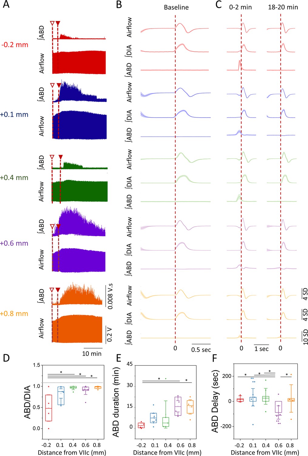
Temporal characteristics of the ABD response elicited after bicuculline injection.
(A) Representative examples of raw traces of the airflow and ∫ABD EMG signals for the entire duration of the response obtained at each injection site following the first (open triangle) and second injection (closed triangle) of bicuculline (examples are color coded based on the groups obtained in Figure 2B). (B–C) Representative mean-cycles for the airflow, ∫DIA EMG, and ∫ABD EMG during baseline (B) and during the first 2 min and the last 2 min of the response (C) (traces are color coded based on the groups defined in Figure 2B). Shaded areas indicate standard deviation of each signal. (D) Coupling of the ∫ABD EMG and ∫DIA EMG following the injection of bicuculline at different rostro-caudal locations. (E) Duration of the ABD response elicited. (F) Delay in the onset of the ABD response following the second injection of bicuculline. Sample size for plots on D–F are as follows: –0.2 mm, n=5; +0.1 mm, n=7; +0.4 mm, n=5; +0.6 mm, n=6; +0.8 mm, n=5. Boxplots represent the median, interquartile range, as well as the minimum and maximum values. Significance levels were obtained through a one-way analysis of variance (ANOVA) followed by a Tukey test, p<0.005. ABD, abdominal; DIA, diaphragm; EMG, electromyogram.
-
Figure 3—source data 1
Temporal characteristics of the abdominal (ABD) response elicited after bicuculline injection (data points for traces presented in Figure 3B and C).
- https://cdn.elifesciences.org/articles/94276/elife-94276-fig3-data1-v1.xlsx
-
Figure 3—source data 2
Temporal characteristics of the abdominal (ABD) response elicited after bicuculline injection (Figure 3D–F dataset).
- https://cdn.elifesciences.org/articles/94276/elife-94276-fig3-data2-v1.xlsx
Figure 4
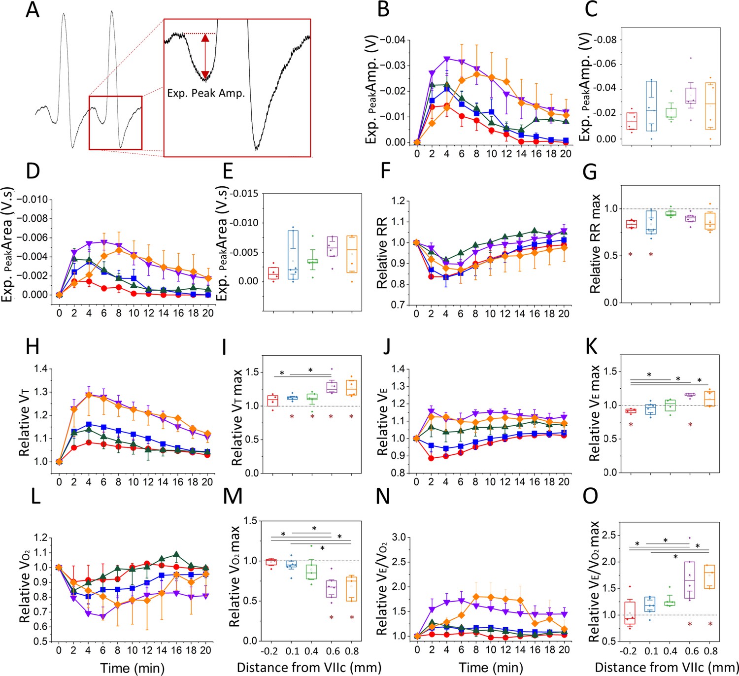
Respiratory changes elicited following bicuculline injection.
(A) Airflow trace depicting the late-expiratory (late-E) inward airflow inflection induced during abdominal (ABD) recruitment, as well as the measure of expiratory peak amplitude used in B. (B, D) Expiratory peak amplitude (B) and area (D), throughout the duration of the post-injection period for each group (color coded based on Figure 2B). Values represent the mean ± SEM at each time bin. (C, E) Maximum expiratory peak amplitude (C) and area (E) obtained at each injection site. (F, H, J, L, N) Relative change in respiratory rate (F), tidal volume (H), minute ventilation (J), oxygen consumption (L), and VE/VO2 (N) with respect to baseline throughout the duration of the post-injection period for each group (color coded based on Figure 2B). Values represent the mean ± SEM at each time bin. (G, I, K, M, O) Maximum relative change in respiratory rate (G), tidal volume (I), minute ventilation (K), oxygen consumption (M), and VE/VO2 (O) observed at each injection site. Sample size for plots on B–O are as follows: –0.2 mm, n=5; +0.1 mm, n=7; +0.4 mm, n=5; +0.6 mm, n=6; +0.8 mm, n=5. Boxplots represent the median, interquartile range, as well as the minimum and maximum values. Significance levels were obtained through a one-way repeated measures analysis of variance (ANOVA) followed by a Bonferroni test, p<0.005 (black asterisks represent significant comparisons between injection sites, red asterisks represent significant comparisons relative to baseline).
-
Figure 4—source data 1
Respiratory changes elicited following bicuculline injection (Figure 4 dataset).
- https://cdn.elifesciences.org/articles/94276/elife-94276-fig4-data1-v1.xlsx
Figure 5
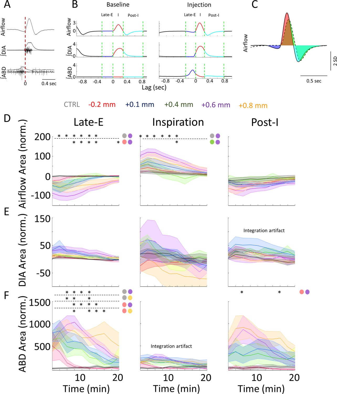
Rostral injections elicit more prominent changes to respiration in each signal and sub-period.
(A-C) Is the same as Figure 1, (Figure 1—source data 1), it has been included here for further clarity when analyzing the results. (A) Raw and integrated EMG activity relative to the onset of inspiration (vertical line). (B) Representative mean-cycles during the baseline and post-injection, defining the late-expiratory (late-E) (blue), inspiratory (red), and post-inspiratory (post-I) (cyan) periods. (C) Sample calculation of normalized area during each phase. (D–F) Normalized response area across post-injection time for the airflow (D), ∫DIA EMG (E), and ∫ABD EMG (F) signals following bicuculline injections into various coordinates along the rostral-caudal axis (colors as per label above figure). Sample size for plots on D–F are as follows: CTRL, n=7; –0.2 mm, n=5; +0.1 mm, n=7; +0.4 mm, n=5; +0.6 mm, n=6; +0.8 mm, n=5. Stars indicate a significant difference (p<0.05) between the responses elicited by different injection locations (color coded based on the groups defined in Figure 2B) as assessed via Kruskal-Wallis test. Colored circles indicate the comparisons which were significant as per Dunn’s post hoc test with Sidak’s correction. Shaded areas indicate mean + SEM. ABD, abdominal; DIA, diaphragm; EMG, electromyogram.
-
Figure 5—source data 1
Rostral injections elicit more prominent changes to respiration in each signal and sub-period, dataset for Figure 5D–F.
- https://cdn.elifesciences.org/articles/94276/elife-94276-fig5-data1-v1.xlsx
Figure 6 with 5 supplements
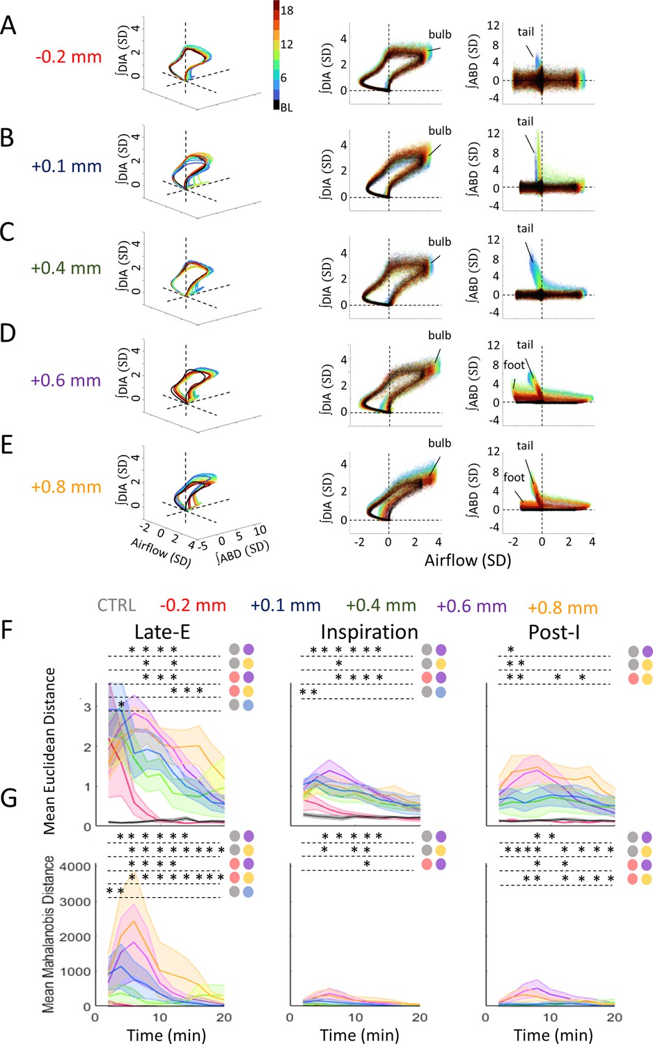
Deformations in multivariate respiratory trajectories differentiate the responses of various rostro-caudal coordinates following bicuculline injections.
(A–E) Representative respiratory trajectories from each injection location. Each row shows the 3D trajectories (solid lines) of the mean-cycle computed for baseline (black) and response time bins (blue to red), based on the color legend in the 3D panel of A. 2D projections of these trajectories onto the airflow-∫DIA EMG (middle), and airflow-∫ABD EMG planes (right) follow on the right of each 3D figure. Clouds of colored points surrounding each trajectory indicate values from individual cycles of the corresponding time bin. Dashed lines indicate the origin of each axis. (F) Mean Euclidean distance across response time bins comparing each injection location for the late-expiratory (late-E), inspiratory, and post-inspiratory (post-I) phases. Colors as per Figure 5, noted above the figure. Shaded areas indicate mean ± SEM. Stars indicate significance (p<0.05) for a given time bin between injection locations or control injections as determined by Kruskal-Wallis test. Colored circles indicate which groups were significantly different as per Dunn’s post hoc testing with Sidak’s correction. (G) Mean Mahalanobis distance across the post-injection response for each injection location and respiratory phase. Colors as in F. Sample size for plots on F–G are as follows: CTRL, n=7; –0.2 mm, n=5; +0.1 mm, n=7; +0.4 mm, n=5; +0.6 mm, n=6; +0.8 mm, n=5. Shaded areas indicate mean ± SEM. Stars indicate significance at the p=0.05 level between injection locations for a given time bin as determined by Kruskal-Wallis test. Colored circles indicate which groups were significantly different as per Dunn’s post hoc with Sidak’s correction. ABD, abdominal; DIA, diaphragm; EMG, electromyogram.
-
Figure 6—source data 1
Deformations in multivariate respiratory trajectories differentiate the responses of various rostro-caudal coordinates following bicuculline injections.
- https://cdn.elifesciences.org/articles/94276/elife-94276-fig6-data1-v1.xlsx
Figure 6—animation 1
Rotating 3D respiratory trajectories highlight the features of breathing in baseline and response conditions.
Trajectories from the sample recordings in Figure 6A (–0.2 mm) across baseline and response time bins (colored as per color bar on right). Each dot represents a timepoint from a given time bin. A subsample of ~11,000 timepoints from each time bin have been randomly selected and are rotated about the diaphragm (DIA) axis to highlight the architecture of respiratory trajectories. Dashed lines indicate the origin of each axis. Axis values expressed in units of standard deviation (SD) as per Methods description.
Figure 6—animation 2
Rotating 3D respiratory trajectories highlight the features of breathing in baseline and response conditions.
Trajectories from the sample recordings in Figure 6B (+0.1 mm) across baseline and response time bins (colored as per color bar on right). Each dot represents a timepoint from a given time bin. A subsample of ~11,000 timepoints from each time bin have been randomly selected and are rotated about the diaphragm (DIA) axis to highlight the architecture of respiratory trajectories. Dashed lines indicate the origin of each axis. Axis values expressed in units of standard deviation (SD) as per Methods description.
Figure 6—animation 3
Rotating 3D respiratory trajectories highlight the features of breathing in baseline and response conditions.
Trajectories from the sample recordings in Figure 6A–C (+0.4 mm) across baseline and response time bins (colored as per color bar on right). Each dot represents a timepoint from a given time bin. A subsample of ~11,000 timepoints from each time bin have been randomly selected and are rotated about the diaphragm (DIA) axis to highlight the architecture of respiratory trajectories. Dashed lines indicate the origin of each axis. Axis values expressed in units of standard deviation (SD) as per Methods description.
Figure 6—animation 4
Rotating 3D respiratory trajectories highlight the features of breathing in baseline and response conditions.
Trajectories from the sample recordings in Figure 6D (+0.6 mm) across baseline and response time bins (colored as per color bar on right). Each dot represents a timepoint from a given time bin. A subsample of ~11,000 timepoints from each time bin have been randomly selected and are rotated about the diaphragm (DIA) axis to highlight the architecture of respiratory trajectories. Dashed lines indicate the origin of each axis. Axis values expressed in units of standard deviation (SD) as per Methods description.
Figure 6—animation 5
Rotating 3D respiratory trajectories highlight the features of breathing in baseline and response conditions.
Trajectories from the sample recordings in Figure 6E (+0.8 mm) across baseline and response time bins (colored as per color bar on right). Each dot represents a timepoint from a given time bin. A subsample of ~11,000 timepoints from each time bin have been randomly selected and are rotated about the diaphragm (DIA) axis to highlight the architecture of respiratory trajectories. Dashed lines indicate the origin of each axis. Axis values expressed in units of standard deviation (SD) as per Methods description.
Additional files
Download links
A two-part list of links to download the article, or parts of the article, in various formats.
Downloads (link to download the article as PDF)
Open citations (links to open the citations from this article in various online reference manager services)
Cite this article (links to download the citations from this article in formats compatible with various reference manager tools)
Mapping responses to focal injections of bicuculline in the lateral parafacial region identifies core regions for maximal generation of active expiration
eLife 13:RP94276.
https://doi.org/10.7554/eLife.94276.3


