A double dissociation between semantic and spatial cognition in visual to default network pathways
- Department of Psychology, University of York, United Kingdom
- York Neuroimaging Centre, Innovation Way, Heslington, United Kingdom
- School of Human and Behavioural Sciences, Bangor University, Gwynedd, Wales, UK, United Kingdom
- Sussex Neuroscience, School of Psychology, University of Sussex, United States
- Department of Psychiatry and Behavioral Sciences, Stanford University School of Medicine Stanford, United Kingdom
- University of Bordeaux, CNRS, CEA, IMN, France
- Brain Connectivity and Behaviour Laboratory, Sorbonne Universities, France
- Department of Psychology, Liverpool John Moores University, United Kingdom
- Integrative Neuroscience and Cognition Center (UMR 8002), Centre National de la Recherche Scientifique (CNRS) and Université de Paris, France
- Department of Psychology, Queen’s University, Kingston, Canada
Figures
Figure 1

Behavioural results for the semantic and spatial context tasks inside the scanner.
SCB = same-category buildings: all the items in the building were taken from the same semantic category. MCB = mixed-category buildings: the items in the buildings were drawn from different semantic categories.
Figure 2 with 1 supplement
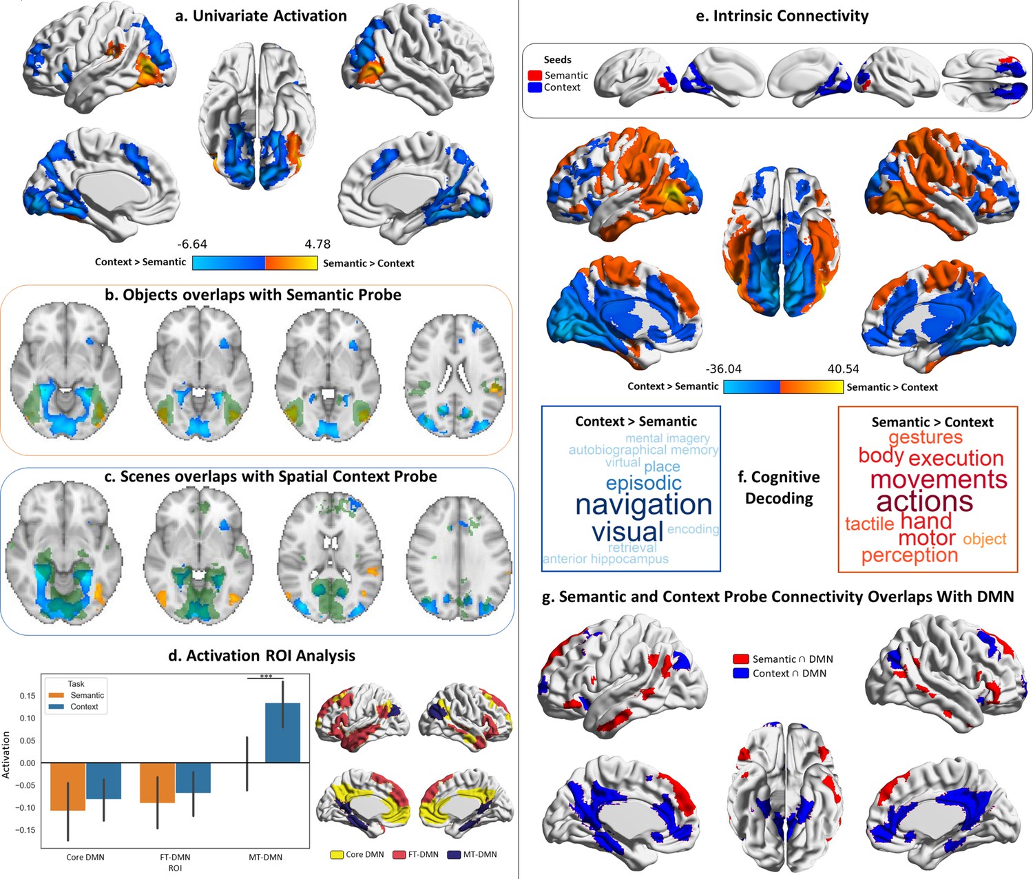
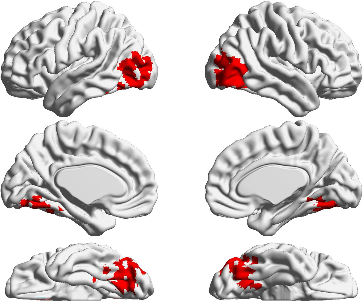
Probe responses.
Warm colours = semantic > spatial context probes. Cool colours = spatial context > semantic probes. Left panel: Univariate results from Study 1, contrasting semantic and spatial context probes. Right panel: Intrinsic connectivity results from Study 3 using semantic and spatial context probe activation within visual networks as seeds. (a) Brain maps depicting the suprathreshold univariate activation results for the probe phase of the semantic and spatial context tasks. (b and c) Axial slices showing the overlap of these univariate results with scene and object localiser maps from Study 2 (the localiser maps are in green, and the univariate results maps are in warm and cool colours; the localiser maps are shown in Figure 2—figure supplement 1). (d) Region of interest (ROI) analysis examining the activation in the three default mode subnetworks of the Yeo 17 parcellation during the probe phase of the semantic and spatial context tasks. The error bars in the bar plots depict the standard error of the mean (Note: ***p<0.001); the ROIs are shown to the right of the bar plots. (e) Brain maps depicting the seeds and intrinsic connectivity results for the semantic and spatial context probe regions. (f) Word clouds depicting the cognitive decoding of unthresholded connectivity maps for semantic and spatial context probe seeds using Neurosynth (bigger words reflect stronger correlation of the functional maps with the terms); the colour code follows that of the brain maps. (g) Brain maps showing the overlap of these intrinsic connectivity maps for semantic and spatial context probes with the default mode network from the 7-network parcellation from Yeo et al., 2011.
Figure 2—figure supplement 1
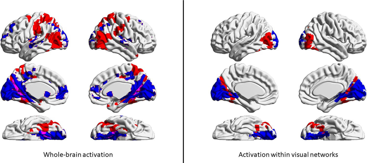
Left panel: Areas associated with the passive viewing of objects are shown in red, and those associated with the passive viewing of scenes are shown in blue; areas that responded to both objects and scenes are shown in purple.
Right panel: The results of the localiser shown in the left panel were further constrained to contain only voxels that overlapped with the visual networks in Yeo’s 17-network parcellation. Common voxels (the ones that responded to both objects and scenes) have been removed.
Figure 3
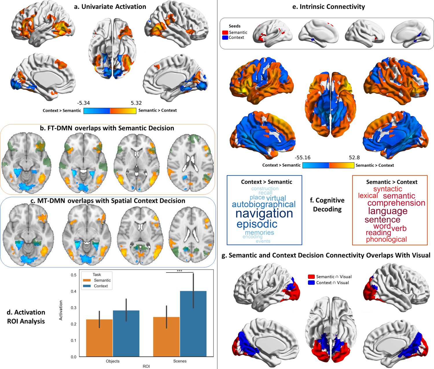
Decision responses.
Warm colours = semantic > spatial context decisions. Cool colours = spatial context > semantic decisions. Left panel: Univariate results from Study 1 contrasting semantic and spatial context decisions. Right panel: Intrinsic connectivity results from Study 3 using semantic and spatial context decision activation within default mode network (DMN) as seeds. (a) Brain maps depicting the suprathreshold univariate activation results for the decision phase of the semantic and spatial context tasks. (b and c) Axial slices showing the overlap of these univariate results with the fronto-temporal (FT) and medial temporal (MT) default mode subnetworks of the Yeo’s 17-network parcellation (the default mode maps are in green, and the univariate results maps are in warm and cool colours). (d) Region of interest (ROI) analysis examining the activation in the scene and object localiser maps from Study 2 during the decision phase of the semantic and spatial context tasks. The error bars in the bar plots depict the standard error of the mean (Note: ***p<0.001, *p<0.05); the ROIs are shown in Figure 2—figure supplement 1. (e) Brain maps depicting the seeds and intrinsic connectivity results for the semantic and spatial context decision regions. (f) Word clouds depicting the cognitive decoding of unthresholded connectivity maps for semantic and spatial context decision seeds using Neurosynth (bigger words reflect stronger correlation of the functional maps with the terms); the colour code follows that of the brain maps. (g) Brain maps showing the overlap of these intrinsic connectivity maps with the visual network from the 7-network parcellation from Yeo et al., 2011.
Figure 4 with 4 supplements
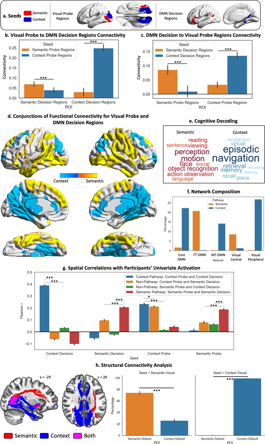
Visual to Default Network Pathways.
(a–c) These panels depict the seeds, regions of interest (ROIs), and their connectivity. The bar plots in (b and c) show the connectivity between default mode network (DMN) decision regions and probe visual regions. (d) Warm colours = common regions showing stronger intrinsic connectivity to semantic decision regions in DMN and semantic probe regions in visual cortex; cool colours = common regions showing stronger intrinsic connectivity to spatial context decision regions in DMN and spatial context probe regions in visual cortex. (e) The cognitive decoding of these spatial maps using Neurosynth following the same colour code as (d). (f) Network composition showing the percentage of each pathway map overlapping with the three DMN and two visual subnetworks defined by the Yeo et al., 2011, 17-network parcellation. (g) Results of spatial correlation analysis comparing the semantic and spatial context pathways with non-pathway maps (derived from the conjunction of the connectivity of probe and decision seeds across different tasks, e.g., probe spatial context ∩ decision semantic connectivity). We assessed the spatial similarity of these pathway and non-pathway maps to the univariate activation during the probe and decision phases for each task and each participant. (h) Results of the structural connectivity analysis. Tracts displayed are a conjunction of streamlines between the probe and decision seeds of each task. The y axis of the bar plots shows the percentage of streamlines from each visual seed that terminate in each DMN ROI (shown in the x axis). The error bars depict the standard error of the mean. ***p<0.001, *p<0.05.
Figure 4—figure supplement 1
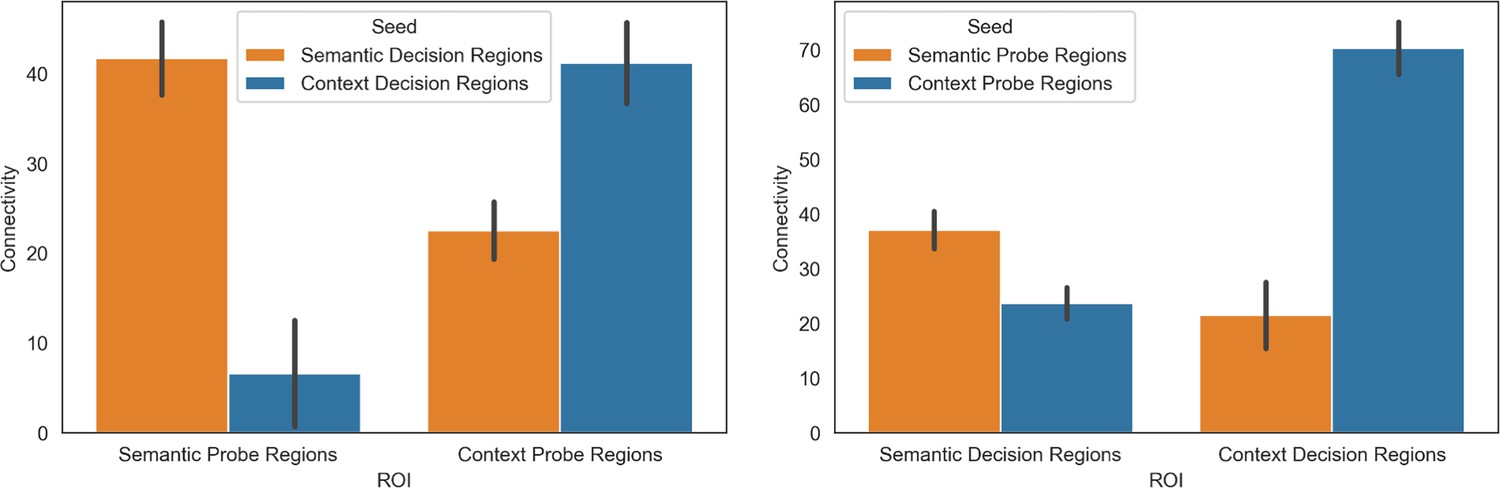
Results of the re-analysis of intrinsic connectivity between semantic and context visual probe and default mode network (DMN) decision regions.
Figure 4—figure supplement 2
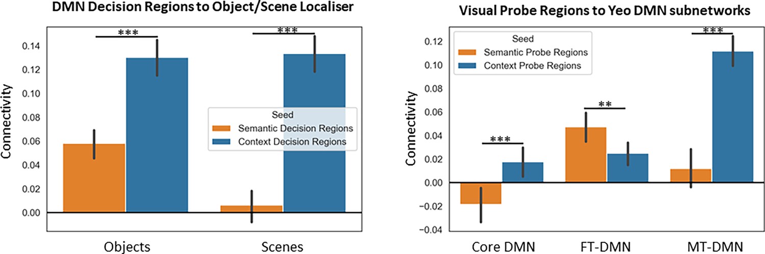
Connectivity of the default mode network (DMN) decision regions to the object/scene localiser from Study 2, and that of the visual probe regions to fronto-temporal (FT), medial temporal (MT), and core DMN of Yeo’s 17-network parcellation.
Figure 4—figure supplement 3
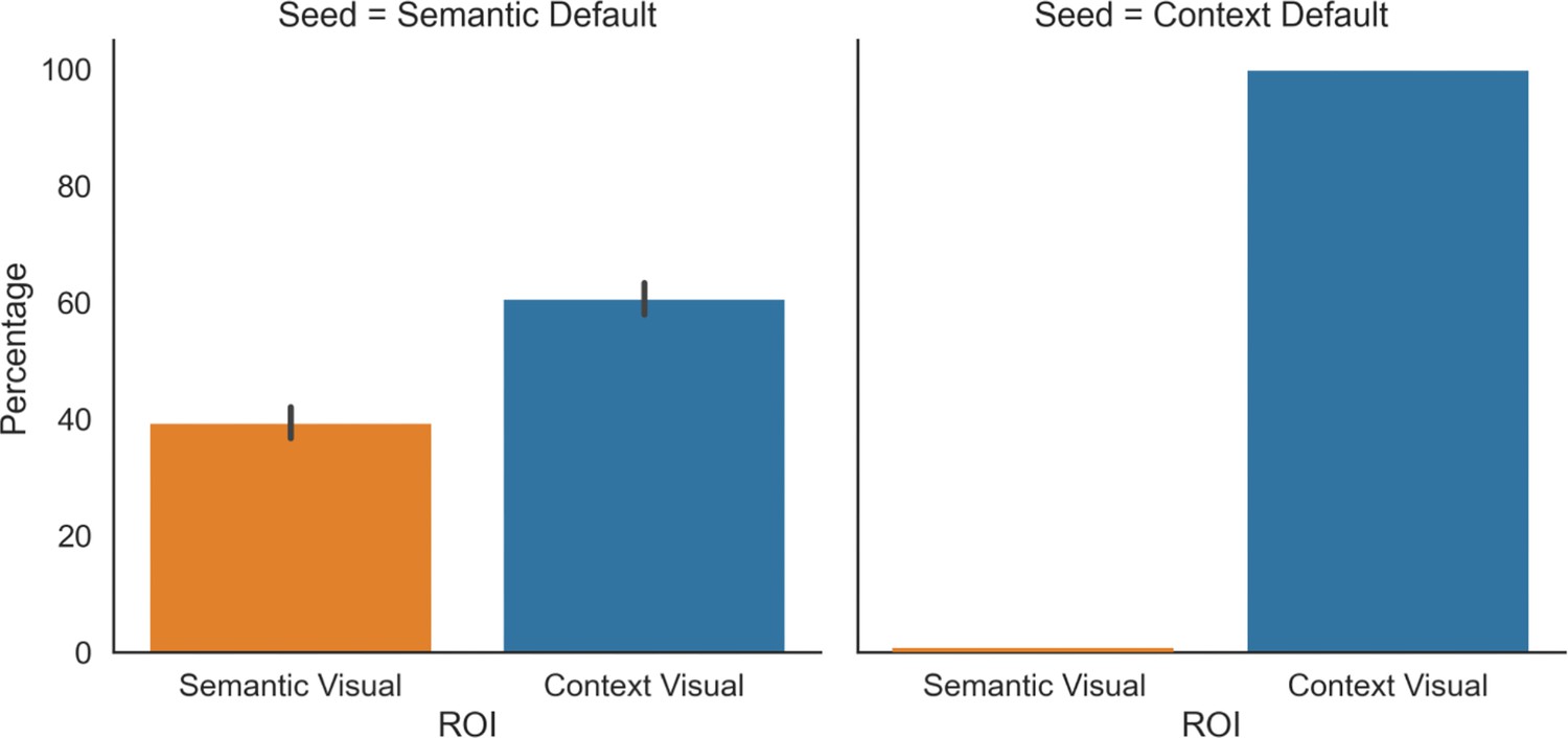
The y axis of the bar plots shows the percentage of streamlines from each default mode network (DMN) seed that terminate in each visual region of interest (ROI) (shown in the x axis).
Seeds and ROIs can be consulted in Figure 4a. The error bars depict the standard error of the mean.
Figure 4—figure supplement 4
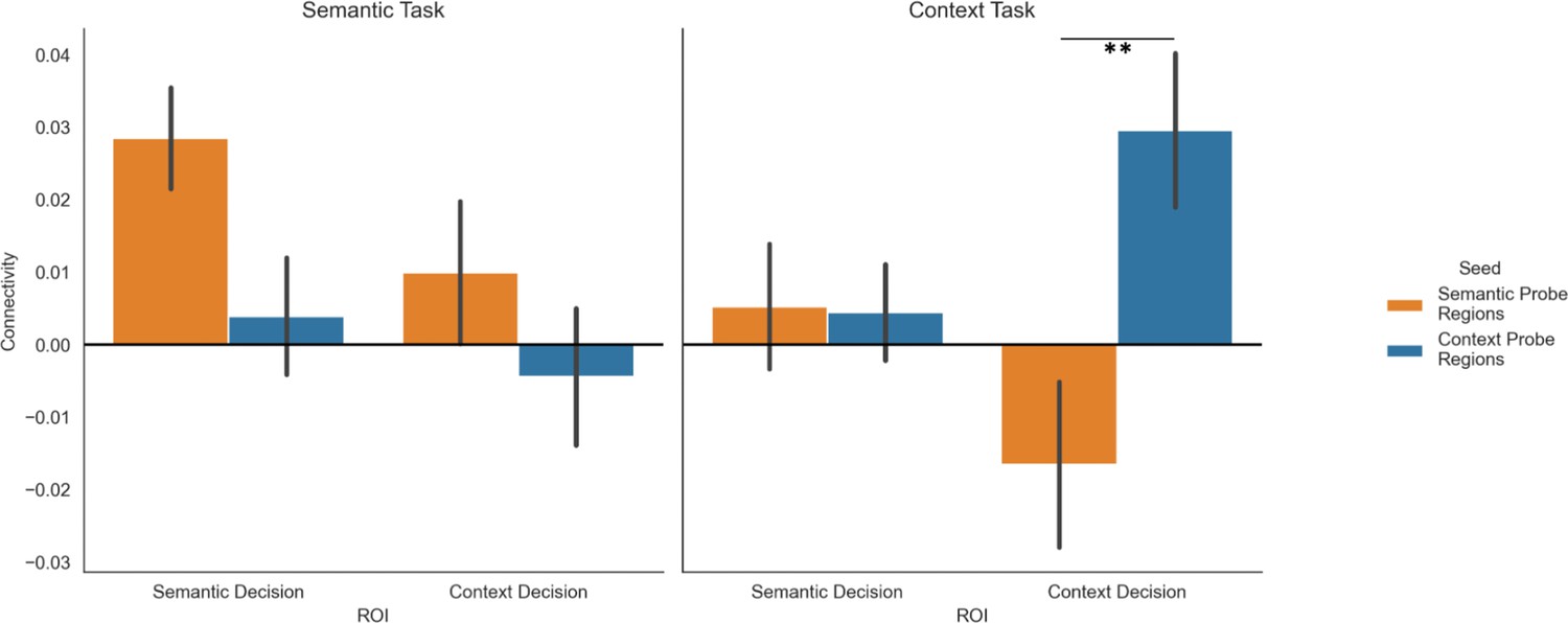
Psychophysiological interaction analysis of the connectivity from the spatial context and semantic probe regions to fronto-temporal (FT) and medial temporal (MT)-default mode network (DMN) subnetworks.
This analysis collapses the same-category building (SCB) and mixed-category building (MCB) conditions, which showed no significant differences. Note: *=p<0.05, **=p<0.01.
Figure 5 with 1 supplement
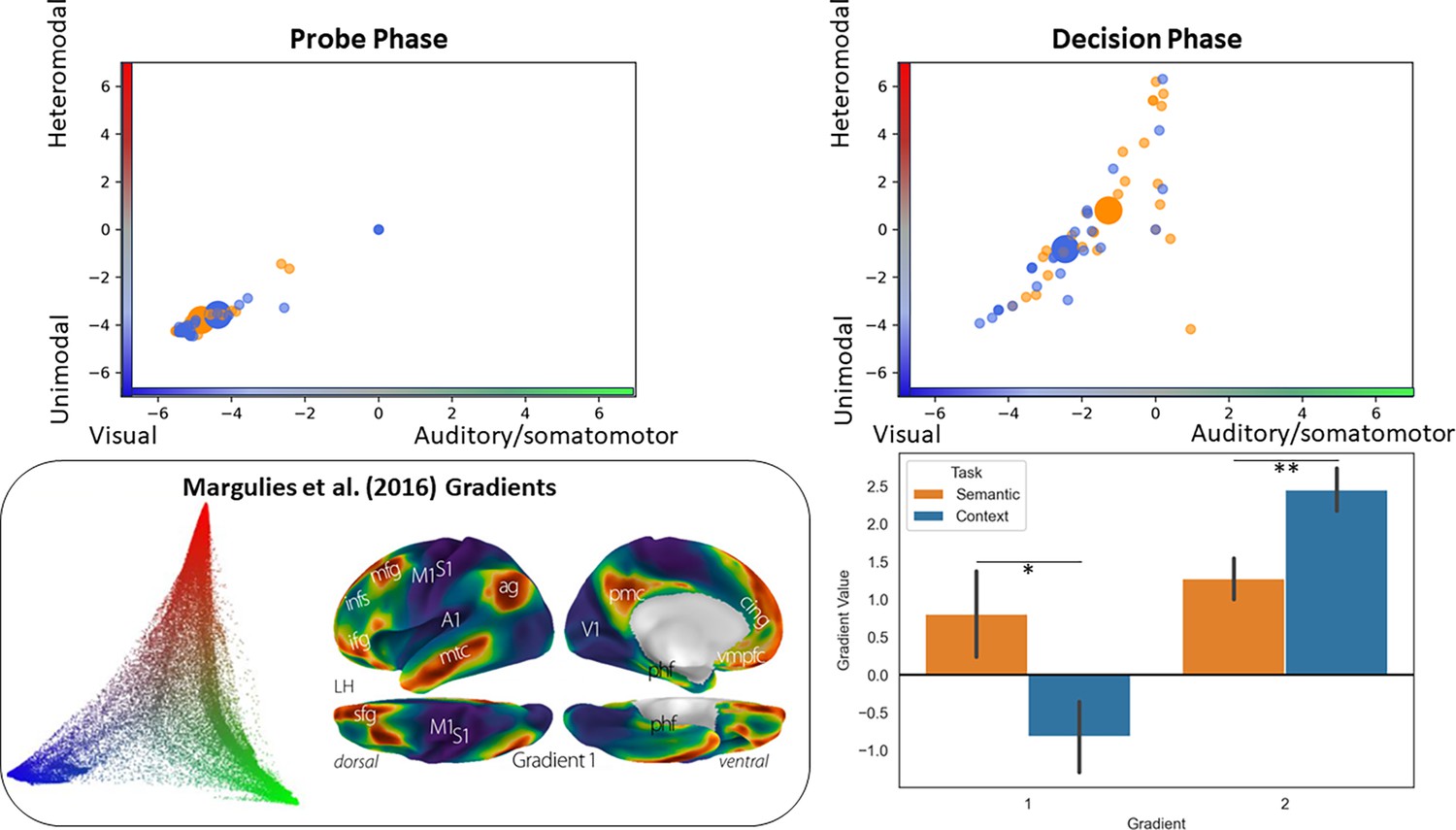
Analysis situating the position of the pathways in a whole-brain connectivity gradient space (Margulies et al., 2016).
The scatterplots depict the position of each participant’s peak response to the semantic and context task in this gradient space (the big circles represent the mean of each task for that phase). The bar plots compare the mean of each gradient across tasks. The inset on the bottom left of the panel displays Margulies et al., 2016, original gradient space.
Figure 5—figure supplement 1
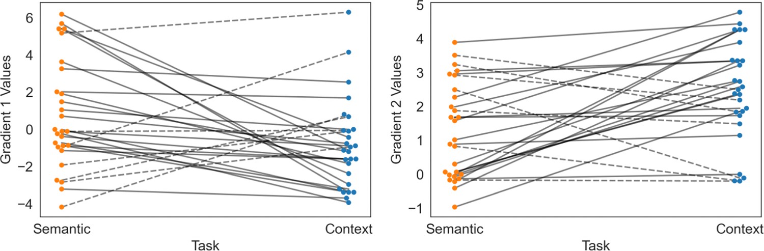
Location in the two principal gradients of the peak response per participant for semantic and spatial context decisions.
Dashed lines highlight the cases that contradict the pattern found in the group-level analysis.
Figure 6 with 2 supplements
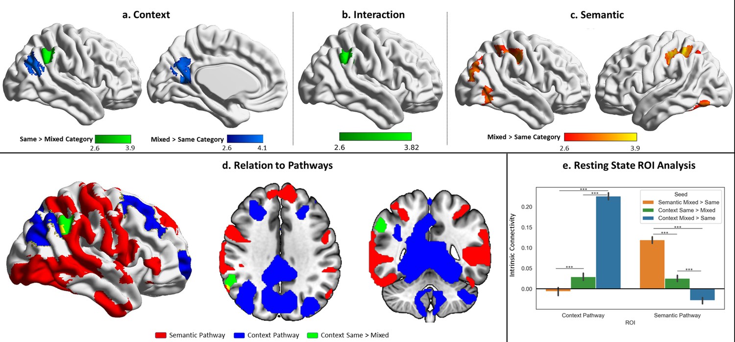
Univariate results for the probe phase contrasting same-category versus mixed-category trials separately for the semantic and spatial context tasks.
(a) Contrast of spatial context same- > mixed-category building trials during the probe phase. (b) Task by condition (same/mixed-category building) interaction. (c) Contrast of semantic same- > mixed-category building trials during the probe phase. (d) Spatial relations of the same > mixed spatial context cluster with the semantic and spatial context pathways outlined in Figure 4. (e) Intrinsic connectivity seed-to-region of interest (ROI) results using the three univariate results clusters shown in the top panel as seeds and the pathways as ROIs. The error bars depict the standard error of the mean. ***p<0.001.
Figure 6—figure supplement 1
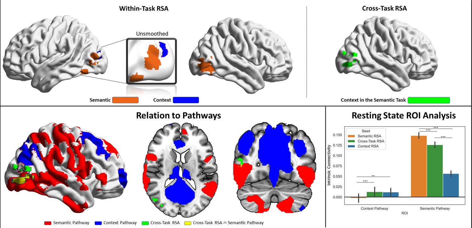
Results of the representational similarity analysis (RSA).
Top left panel: Within-task RSA results correlating BOLD activity from the probe phase of semantic mixed-category building trials with the semantic similarity matrix described in the Methods section, and BOLD activity from the probe phase of context mixed-category building trials with the context similarity matrix. Top right panel: Cross-task similarity analysis correlating BOLD activity from semantic trials with the context similarity matrix. Bottom panel: The left part depicts the spatial relations of the cross-task similarity analysis cluster with the semantic and context pathways outlined in Figure 4; the right part shows intrinsic connectivity seed-to-region of interest (ROI) results using the within- and cross-task RSA clusters shown in the top panel as seeds and the pathways as ROIs. The error bars depict the standard error of the mean. ***p<0.001, **p<0.01.
Figure 6—figure supplement 2
Representational similarity analysis results for the same-category building trials of the probe phase of the semantic task.
No significant voxels were identified for the spatial context task.
Figure 7 with 2 supplements
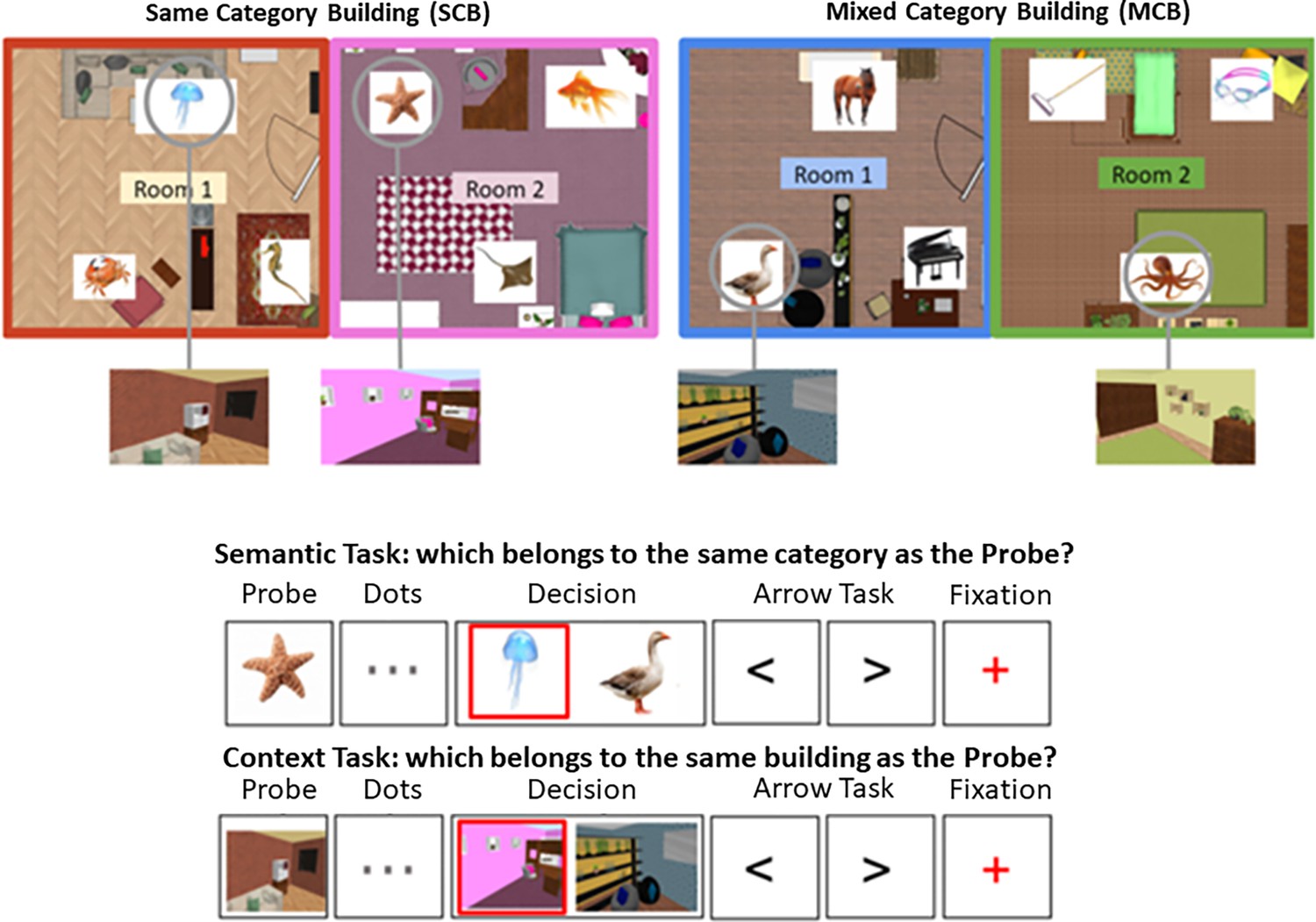
Top panel: the layout of two buildings is shown, one of them contains semantically related items (same-category building [SCB]), the other contains unrelated items (mixed-category building [MCB]).
These items and locations are shown in the example trials below. Bottom panel: Trial procedure for semantic and spatial context decisions. The phases of a trial are shown (probe, dots, decision, arrow task, fixation), and the red square indicates the correct response (not shown to participants). Participants were required to press ‘left’ or ‘right’ buttons in the decision phase. No-decision trials omitted the dots and decision phases. The videos and tests used during the training session for this task as well as the stimuli used in the task of Study 2 can be consulted in Figure 7—figure supplements 1 and 2.
Figure 7—figure supplement 1
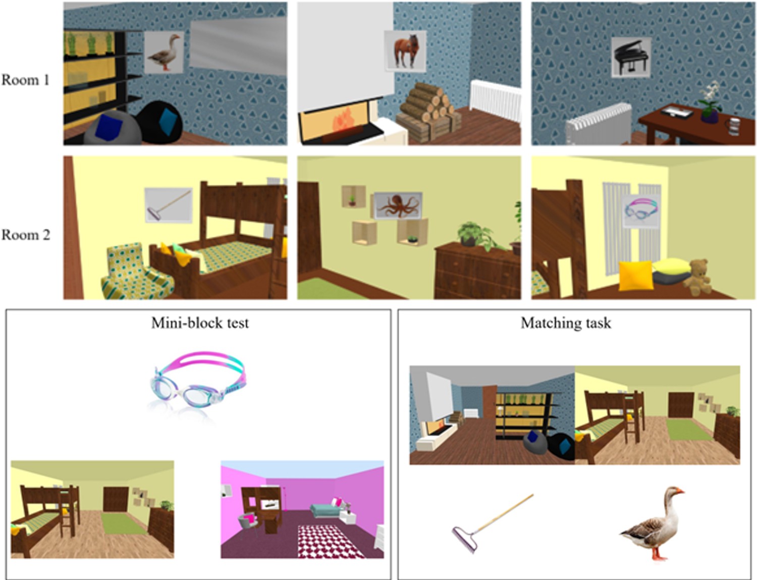
Top panel: An example of what was seen during the training videos.
This is a ‘mixed-category building’ that contains items from different semantic categories. An example walk-through video of this building can be watched following this link: https://www.youtube.com/watch?v=XVHhOh3BF74. Bottom panel: Example of training tests. On the left is an example of the mini-block test depicting the probe item at the top and two room screenshots below. The target screenshot is the room the object was presented in at training (left). The distractor screenshot (right) is from a different building, which the object did not belong to. On the right is an example of the matching task depicting two rooms from the same building and two items that belong to each room (rake-right room, goose-left room) which participants needed to match.
Figure 7—figure supplement 2
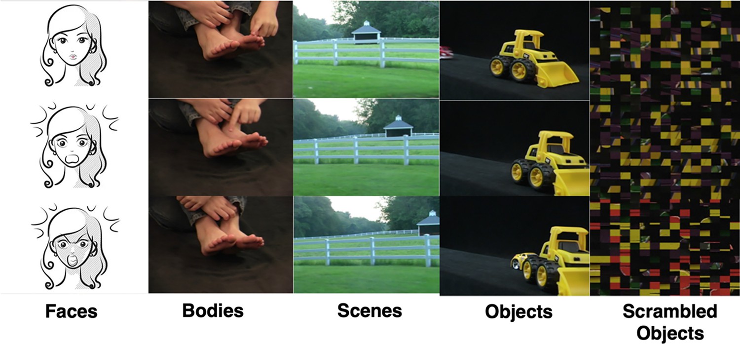
Examples of the dynamic images taken from the 3 s movie clips depicting faces, bodies, scenes, objects, and scrambled objects.
Still images taken from the beginning, middle, and end of the corresponding movie clip. The stimuli corresponding to the ‘faces’ condition were changed to line drawings to make this material suitable for hosting in bioRxiv preprint server. The actual stimuli shown can be consulted in the OSF collection associated with this paper (https://osf.io/sh79m/).
Additional files
-
MDAR checklist
- https://cdn.elifesciences.org/articles/94902/elife-94902-mdarchecklist1-v1.docx
-
Supplementary file 1
Cluster Information for Neuroimaging Results from Study 1.
- https://cdn.elifesciences.org/articles/94902/elife-94902-supp1-v1.docx
-
Supplementary file 2
Paired t-tests contrasting spatial similarity of participant-level activation with group-level context and semantic pathways and non-pathways.
- https://cdn.elifesciences.org/articles/94902/elife-94902-supp2-v1.docx
Download links
A two-part list of links to download the article, or parts of the article, in various formats.
Downloads (link to download the article as PDF)
Open citations (links to open the citations from this article in various online reference manager services)
Cite this article (links to download the citations from this article in formats compatible with various reference manager tools)
A double dissociation between semantic and spatial cognition in visual to default network pathways
eLife 13:RP94902.
https://doi.org/10.7554/eLife.94902.3


