Bridging the 3D geometrical organisation of white matter pathways across anatomical length scales and species
- Danish Research Centre for Magnetic Resonance, Center for Functional and Diagnostic Imaging and Research, Copenhagen University Hospital Amager and Hvidovre, Denmark
- Department of Applied Mathematics and Computer Science, Technical University of Denmark, Denmark
- Guangdong Provincial Engineering Research Center of Molecular Imaging, The Fifth Affiliated Hospital, Sun Yat-sen University, China
- ESRF - The European Synchrotron, France
- Department of Computer Science, University of Verona, Italy
- Institut für Röntgenphysik, Universität Göttingen, Friedrich-Hund-Platz, Germany
- Department of Neurology, Odense University Hospital, Denmark
- Institute of Molecular Medicine, University of Southern Denmark, Denmark
- BRIDGE—Brain Research—Inter-Disciplinary Guided Excellence, Department of Clinical Research, University of Southern Denmark, Denmark
- Rheumatology Research Unit, Odense University Hospital, Denmark
- School of Optometry, University of Montreal, Canada
Figures
Figure 1
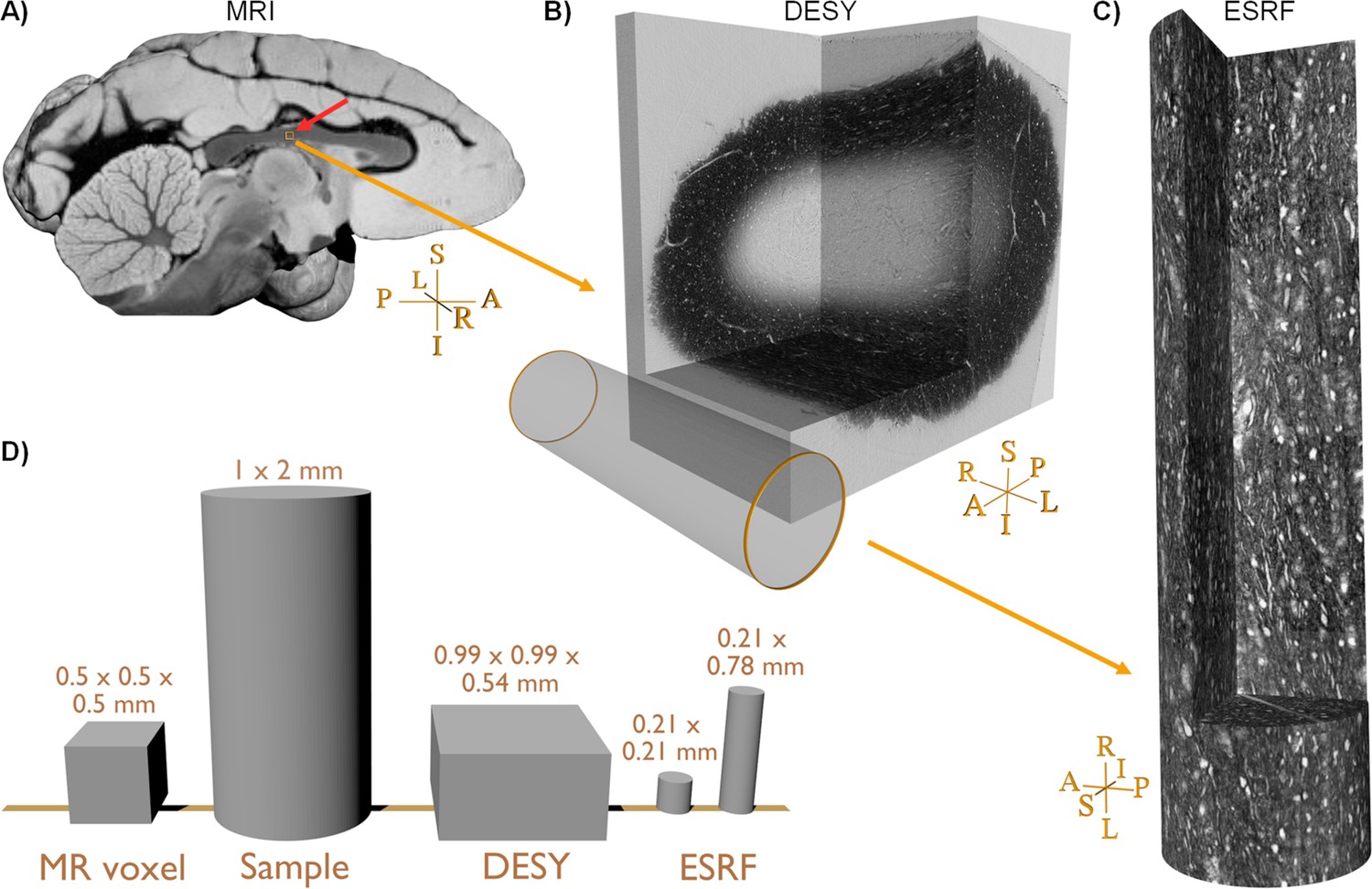
Sample comparison.
(A) Rendering of the vervet monkey brain structural magnetic resonance imaging (MRI) close to the mid-sagittal plane. (B) Large field-of-view (FOV) scanning of the biopsy, Deutsches Elektronen-Synchrotron (DESY). The small orange box near the red arrow in (A) indicates the location and size of the FOV within the MRI data. (C) The stack of four small FOVs scans obtained at European Synchrotron (ESRF). The cylinder in (B) indicates the relative size of the FOV within the DESY scan. (D) Relative size comparison of one MRI voxel, the biopsy sample prior to staining and fixation, and various synchrotron FOVs. For cylindrical FOVs, the first number indicates the diameter, and the second number is the height. Sample orientations are related to the whole brain in (A): R: Right, L: Left, I: Inferior, S: superior, A: Anterior, P: posterior.
Figure 2
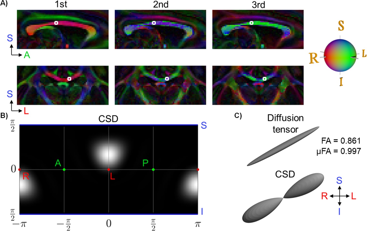
Diffusion magnetic resonance imaging (dMRI)-based orientations and tensor shapes.
(A) The diffusion tensor model showing principal directions in a sagittal slice of the monkey corpus callosum (CC). The voxel corresponding to the biopsy sampling location (the synchrotron field-of-views, FOVs) is outlined in a white box. (B) The fibre orientation distribution (FOD) of the constrained spherical deconvolution (CSD) model in the selected diffusion MRI voxel is represented as a spherical polar histogram. (C) The corresponding glyph representations of the diffusion tensor and CSD.
Figure 3
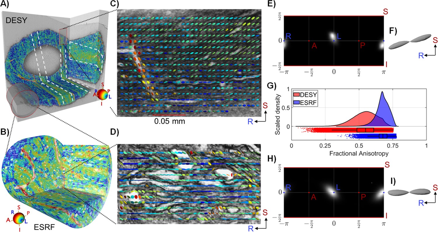
Structure tensor shape for corpus callosum (CC) sample.
(A–B) 3D renderings from respectively the Deutsches Elektronen-Synchrotron (DESY) and European Synchrotron (ESRF) CC biopsy samples with structure tensor main direction colour coding (in accordance with the colour sphere). The white markings illustrate bands where axons are oriented at an angle compared to their surroundings, indicating a laminar organisation. The red cylinder on (A) shows the scale difference between the DESY and ESRF data. The position of the sample within the CC is marked on the MR image in Figures 1A and 2A. (C–D) Selected coronal slice overlaid with a regularly spaced subset of structure tensor glyphs, coloured according to their predominant direction. (E–F) Spherical polar histograms of the DESY structure tensor main directions (FOD) and the corresponding glyph. (G) Kernel density estimates of structure tensor fractional anisotropy (FA) values. (H–I) Spherical histogram of the ESRF structure tensor main directions (FOD) and the corresponding glyph. NB: We exclude contributions from the voxel of blood vessels in FA histograms and FODs.
Figure 4 with 1 supplement
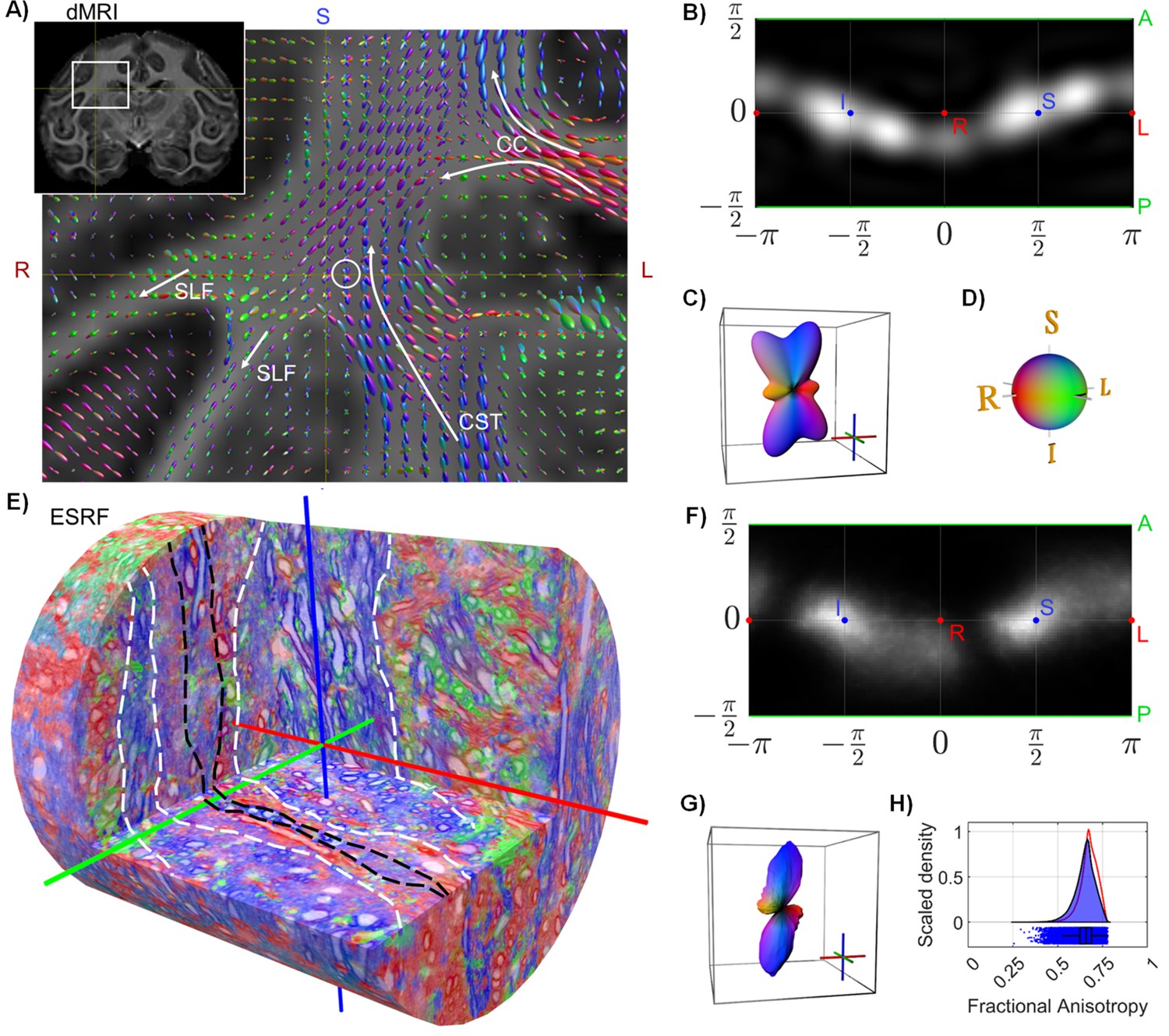
Results in complex monkey deep white matter (WM) region.
A) Anatomy and constrained spherical deconvolution (CSD) glyphs are seen in the volume surrounding the local neighbourhood of the sampled biopsy location (white circle). (B and C) Results in the matching magnetic resonance imaging (MRI) voxel, showing (CSD) fibre orientation distribution (FOD) and the corresponding glyph. (D) The directional colour map used throughout the figure. (E) Example of rendering from an European Synchrotron (ESRF) volume with colouring corresponding to the structure tensor main direction. Marking with dashed lines indicates clear fasciculi. (F and G) Structure tensor directional statistics from the stacked field-of-view (FOV), showing the structure tensor FOD and corresponding glyph. (H) Structure tensor shape statistics from the stacked FOV, showing the kernel density estimate of fractional anisotropy (FA) values. The red curve is a copy of the FA distribution from the ESRF corpus callosum (CC) region (Figure 3G).
Figure 4—video 1
Animation related to Figure 4E.
Rendering of the full stacked monkey European Synchrotron (ESRF) centrum semiovale sample with colouring corresponding to the main direction from structure tensor analysis.
Figure 5 with 2 supplements
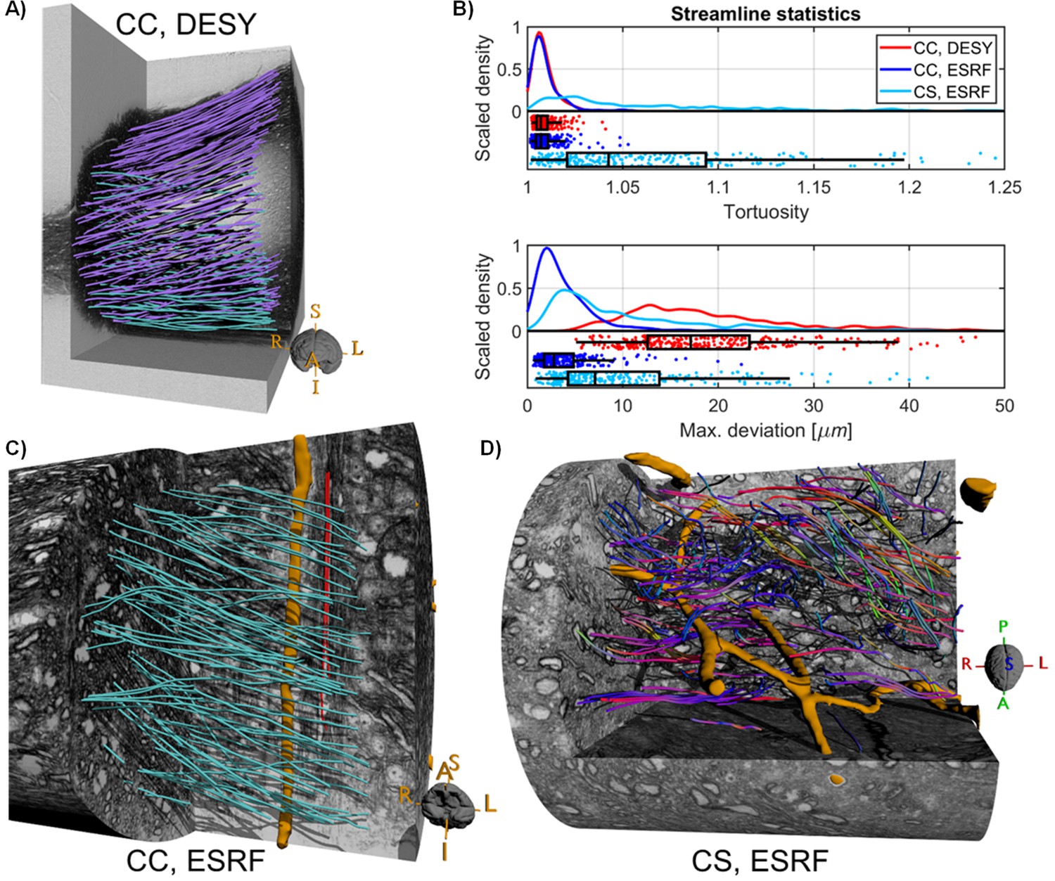
Structure tensor-based tractography for the monkey samples.
(A) Streamlines in the corpus callosum (CC) sample from Deutsches Elektronen-Synchrotron (DESY). Purple streamlines have a strong upward directional component, unlike the cyan streamlines (assuming that streamlines travel from right to left). (B) The statistics of streamlines quantification using tortuosity index and maximum deviation. (C) A selection of streamlined in the CC within a single ESRF scan. Cyan streamlines have R-L as the strongest directional component, whereas red streamlines do not. The orange structure is a segmented blood vessel. (D) Streamlines in the complex centrum semiovale region (CS) within a single ESRF scan. Streamlines are coloured according to their local main direction. Orange structures represent segmented blood vessels.
Figure 5—video 1
Animation related to Figure 5A.
Rendering of structure tensor-based streamlines in the monkey Deutsches Elektronen-Synchrotron (DESY) corpus callosum sample from varied viewpoints. Purple streamlines have a strong upwards directional component, unlike the cyan streamlines (assuming that streamlines travel from right to left). Orange structures represent segmented blood vessels.
Figure 5—video 2
Animation related to Figure 5D.
Rendering of structure tensor-based streamlines in the complex centrum semiovale region within a single European Synchrotron (ESRF) scan from the monkey. Streamlines are coloured according to their local main direction. Orange structures represent segmented blood vessels.
Figure 6
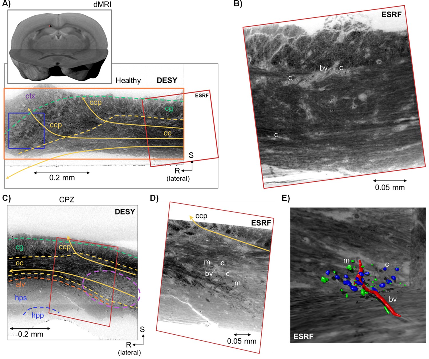
Overview of the mouse datasets.
(A) Location of the sample within the mouse brain and a coronal slice from the Deutsches Elektronen-Synchrotron (DESY) dataset, with indications of anatomic regions: cc = corpus callosum, cg = cingulum, ctx = cortex, and ccp = cortical projections. The blue box indicates the size of a DWI voxel. (B) The co-registered slice from the European Synchrotron (ESRF) volume (position indicated by the red frame). Labels indicating blood vessels (bv) and cells (c), (C) Coronal slice from the DESY dataset of a cuprizone (CPZ)-treated mouse, with indication of anatomic regions: cc = corpus callosum, cg = cingulum, alv = alveus, hps = hippocampal striatum, hpp = hippocampal pyramidal layer, ccp = cortical projections. The dashed purple line shows a demyelinated region of the CC. (D) The co-registered slice from the ESRF volume (indicated by the red frame). Labels indicate blood vessels (bv), cells (c), and myelin ‘debris’/macrophages (m). (E) 3D rendering of a local segmentation in the corresponding region in D. The blood vessel is coloured in red, cells in blue, and ‘myelin debris’ in green. This segmentation was done manually using ITK-SNAP (RRID:SCR_002010).
Figure 7
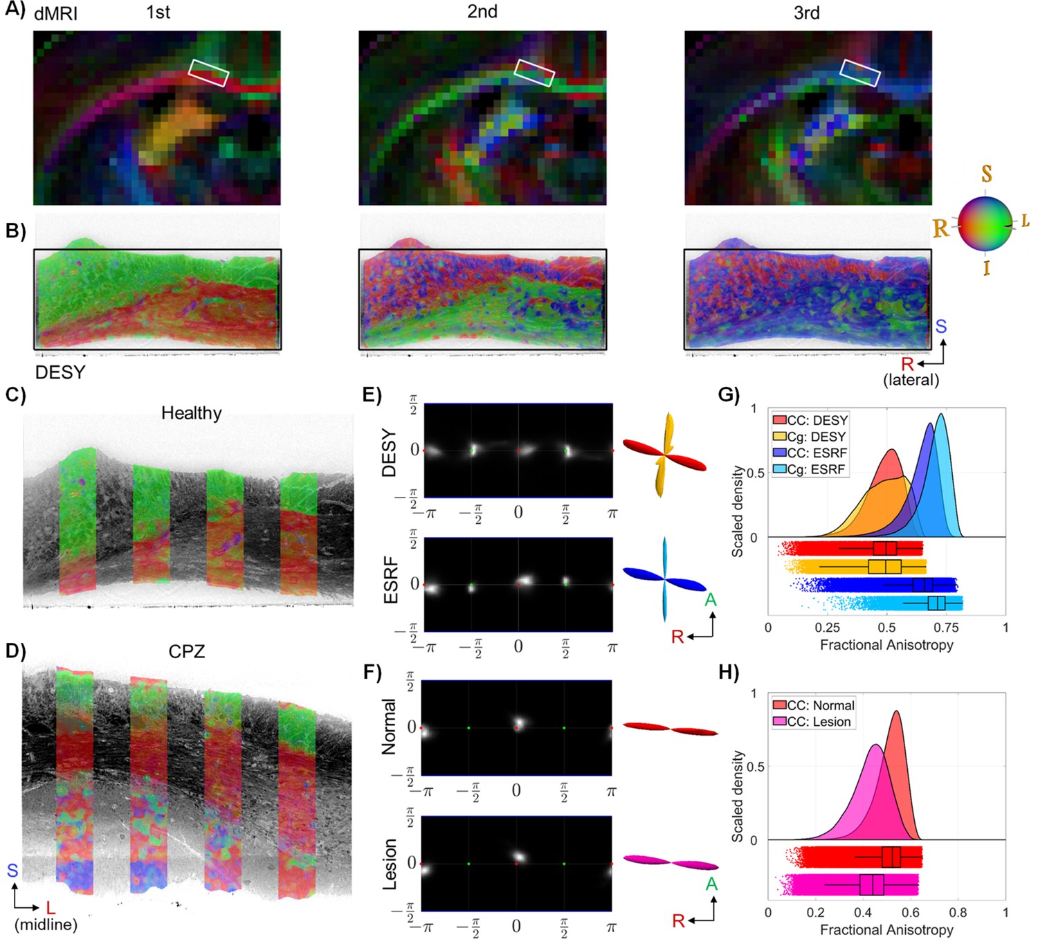
Mouse diffusion tensor and structure tensor results.
(A) and (B): The directional components of the diffusion tensor and the structure tensor in a coronal slice from a healthy mouse brain. The white frame in (A) indicates the approximate size and location of the Deutsches Elektronen-Synchrotron (DESY) field-of-view (FOV), i.e., the black frame in (B). (C) and (D) The main structure tensor direction from the DESY data overlaid on a slice from a healthy mouse brain (C) and a cuprizone (CPZ)-treated mouse (D). (E) Structure tensor fibre orientation distributions (FODs) from a healthy mouse along with corresponding glyphs. The glyph colouring indicates whether the FOD contribution is from the corpus callosum (CC) (red/blue) or cingulum (yellow/cyan). (F) structure tensor FODs from the CPZ-treated mouse CC (DESY), split into contributions from a normal appearing region and a demyelinated area. (G) and (H) structure tensor fractional anisotropy (FA) distributions from various regions of healthy and lesioned mouse samples.
Figure 8
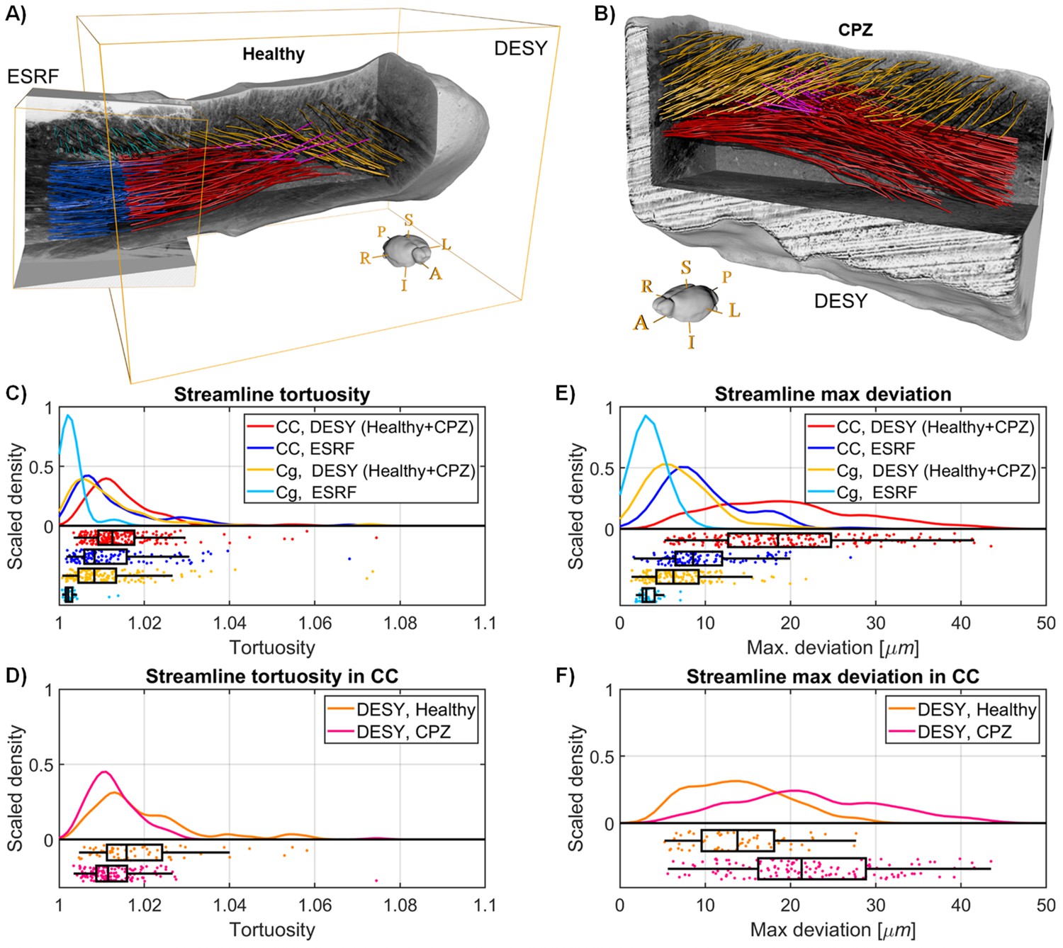
Mouse tractography results.
(A) Tractography visualisation from a healthy mouse brain sample. Red and Blue: Streamlines in corpus callosum (CC). Yellow and Cyan: Streamlines in cingulum. Pink streamlines are extrapolations of CC streamlines that represent plausible cortical projections through the cingulum. (B) Tractography visualisation from Deutsches Elektronen-Synchrotron (DESY) data of a cuprizone (CPZ)-treated mouse brain. (C) and (E) Tractography streamlines centroid statistics from the healthy mouse brain synchrotron volumes. The curves are kernel density estimates of the tortuosity and maximum deviation, respectively. (D) and (F) Statistics for the streamlines in the corpus callosum of the DESY healthy and CPZ mouse brain samples.
Appendix 1—figure 1
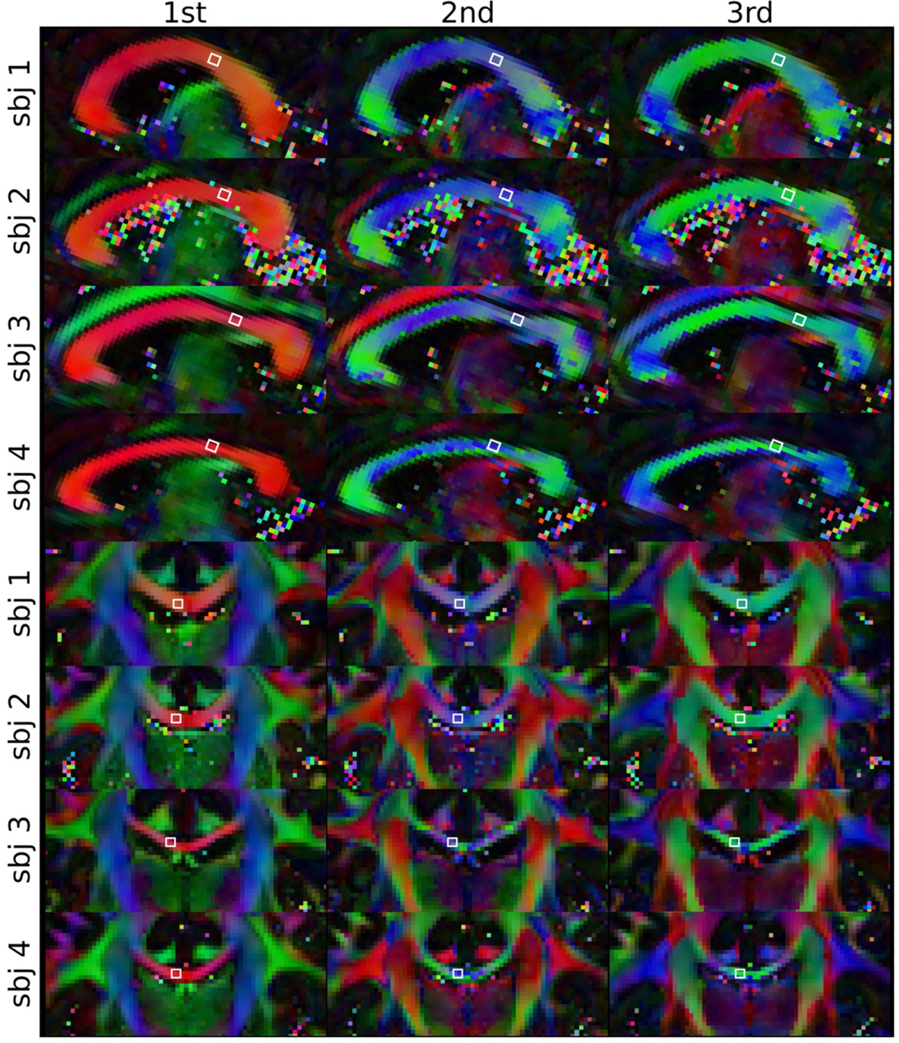
Human Connectome Project (HCP) dataset diffusion tensor modelling.
The RGB colour-coded first, second, and third eigenvectors (ordered by decreasing eigenvalues) for the four subjects in both sagittal and coronal crop-out views.
Appendix 1—figure 2
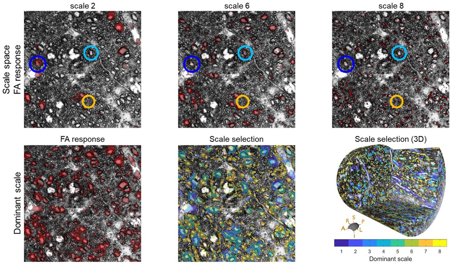
Example of applying the scale-space structure tensor.
(Top row): A region of a slice from the European Synchrotron (ESRF) monkey corpus callosum (CC) sample, where the fractional anisotropy (FA) is estimated from eight scales (see Table 2), here showing only the scales 2, 6, and 8. The red transparent overlay shows the thresholded FA response (FA > 0.7). Notice how large, medium, and small cross-sectional axons respond differently at the different scales (represented by the blue, light blue, and orange circles, respectively). (Bottom row, left): The final thresholded dominant FA response (dFA > 0.7), shows high FA values for all axons regardless of the diameter. (Bottom row, mid and right): The same subset of voxels coloured according to the dominant scale index for the same 2D slice region and in a 3D rendering respectively. Notice how the low scales (large kernels) are selected for large axons, and similarly high scales (small kernels) are selected for the small axons.
Appendix 1—figure 3
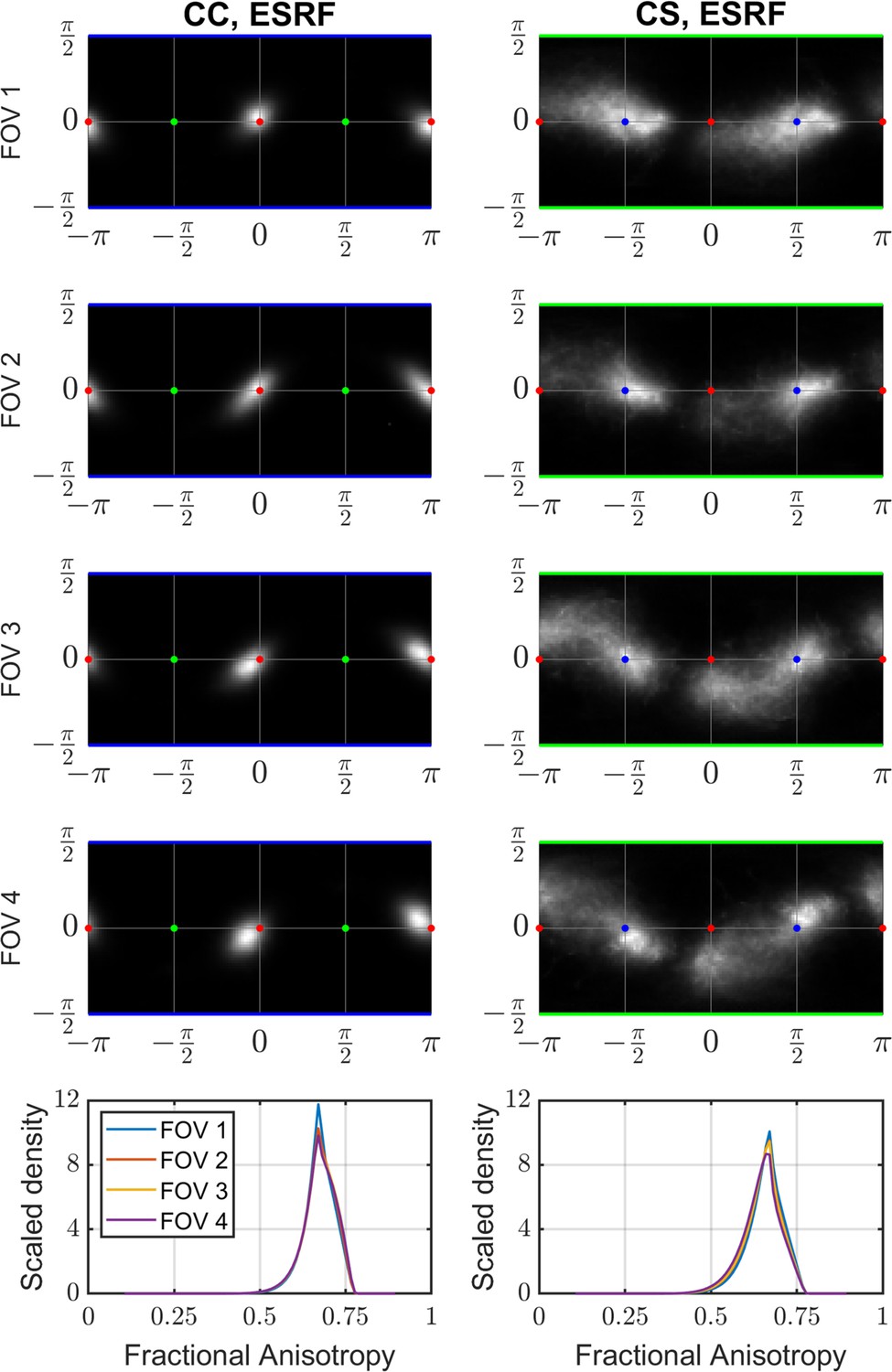
ST-derived statistics from the individual stacked field-of-views (FOVs) in the monkey European Synchrotron (ESRF) corpus callosum (CC) and centrum semiovale (CS) sample.
(Rows 1-4): Individual fibre orientation distributions (FODs) showing minor variation as the FOV placement changes. Across the CC, the most notable change is the anisotropic shape of the peak. Across the CS, the prominence of the L-R directed peak (near the red points) represents the largest variation. (Row 5): FA distributions of the four individual FOVs plotted together, showing almost no difference in the statistics.
Tables
Table 1
Data samples included in this study.
All voxel sizes are isotropic. The field-of-views (FOVs) of ID-2 and ID-3 are given as four stitched scans (marked with *). Individual FOVs were 0.21×0.21×0.21 mm.
| ID | Specimen | Synchrotron | Sample | FOV [mm] | Voxel size [nm] | |
|---|---|---|---|---|---|---|
| 1 2 | Monkey | DESY ESRF | Corpus callosum (CC), midbody | 0.54×0.99 ×0.99 0.78×0.21 ×0.21* | 550 100 | |
| 3 | ESRF | Centrum semiovale (CS) | 0.78×0.21 ×0.21* | 100 | ||
| 4 5 | Mouse | DESY ESRF | Corpus callosum, splenium & cingulum | 0.63×0.35 ×0.35 0.24×0.24 ×0.24 | 550 75 | |
| 6 7 | CPZ Mouse | DESY ESRF | 0.64×0.38 x 0.50 0.30×0.30 ×0.30 | 550 100 |
Table 2
Structure tensor parameter values used for the samples in this study (see Table 1 for sample ID).
The kernel size represents the width of the ρ-kernel converted to physical distance in accordance with the voxel size of the specific dataset. The scale-space approach was applied only to the monkey ESRF samples, with the range of scales listed in Table 2. In all other cases, the image resolution was too low compared to the anatomical scale for structures to visually present with distinguishably different sizes. Therefore, there was no benefit in the scale-space approach. Instead, the standard ST analysis with a fixed kernel size was used.
| ID | Voxel size [nm] | Scaling factor | ST-parameters (ρ,σ) [voxels] | ST conversion (γ) | Kernel size [μm] | |
|---|---|---|---|---|---|---|
| 1 2 | 550 100 | 2 4 | 2.5 8 scales* | 0.5 8 scales* | 0.30 0.30 | 12 [9.2–2] |
| 3 | 100 | 4 | 8 scales* | 8 scales* | 0.30 | [9.2–2] |
| 4 5 | 550 75 | 2 5 | 4 6 | 1 1 | 0.35 0.25 | 18.7 9.4 |
| 6 | 550 | 2 | 4 | 1 | 0.35 | 18.7 |
-
*
Scale space structure tensor parameters:ρ = [5.50, 4.50, 3.50, 3.50, 2.50, 2.50, 1.50, 1.00], σ = [3.00, 2.75, 2.50, 1.50, 1.50, 1.00, 1.00, 0.50].
Download links
A two-part list of links to download the article, or parts of the article, in various formats.
Downloads (link to download the article as PDF)
Open citations (links to open the citations from this article in various online reference manager services)
Cite this article (links to download the citations from this article in formats compatible with various reference manager tools)
Bridging the 3D geometrical organisation of white matter pathways across anatomical length scales and species
eLife 13:RP94917.
https://doi.org/10.7554/eLife.94917.3


