Figures and data in Modeling collective behavior in groups of mice housed under semi-naturalistic conditions

Figures
Tables
Additional files

4 figures, 1 table and 1 additional file

Figures

Figure 1 with 1 supplement

Download asset Open asset

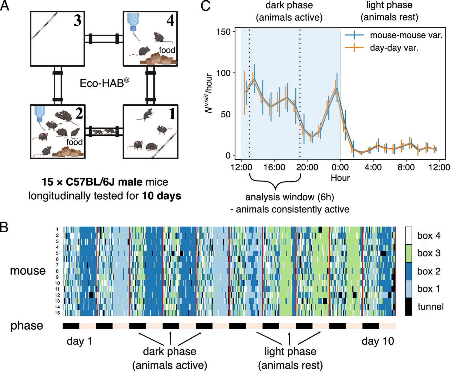
Mice were tested in Eco-HAB, a system for automated, ecologically relevant assessment of voluntary behavior in groups of mice.

Animals were tested for 10 days. (A) Schematic of the Eco-HAB system, where four compartments are connected with tunnels. Food and water are available ad libitum in compartments 2 and 4. (B) Time series of the location of 15 mice over 10 days, as aligned to the daylight cycle. (C) Circadian clock affects the activity of the mice, measured by the number of transitions in each hour averaged over the 15 mice and the 10 days. Error bars represent SD across all mice (mouse-mouse variability, in blue) or across all days for the mean activity level for all mice (day–day variability, in orange). The two curves are slightly shifted horizontally for clearer visualization. We focus the following analysis on the data collected during the first half of the dark phase, between 13:00 and 19:00 (shaded region).

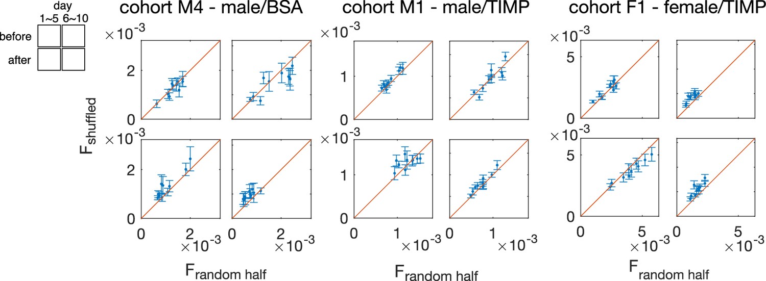
Figure 1—figure supplement 1

Download asset Open asset

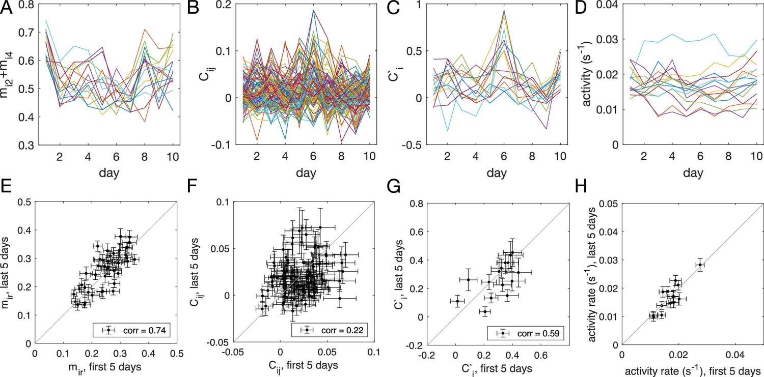
Stability of the data, given by the time evolution across 10 days of the experiment and the scatter plot between the observables measured using the first 5 days of the data versus the last 5 days of the data for cohort M1 ( $N = 15$ ).

The observables plotted include (**A, E**) $m_{i r}$ , probability of mouse $i$ being found in compartment $r$ , (**B, F**) $C_{i j}$ , the (connected) pairwise correlation, or the in-cohort sociability, between mouse $i$ and mouse $j$ , (**C, G**) the sum of observed in-cohort sociability, $C_{i} \equiv Σ_{j \neq i} C_{i j}$ which gives a proxy for how mouse $i$ is effected by the social interaction, and (**D, H**) the activity rate, measured by the number of transition event per second. The error bars in panels (E–H) are extrapolated from random halves of the data.

Figure 2 with 8 supplements

Download asset Open asset

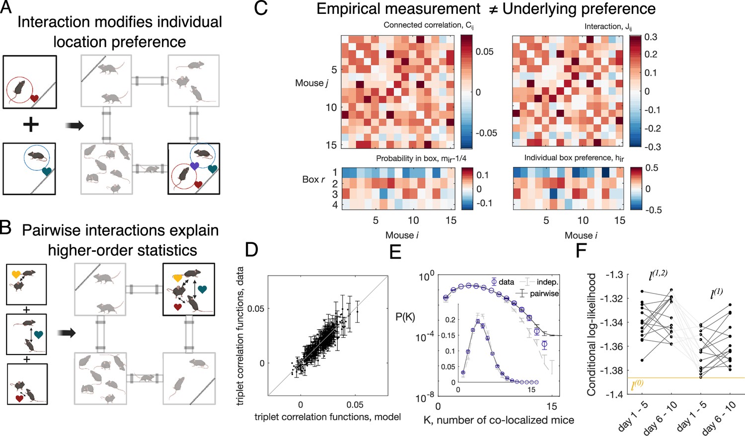
Mice in Eco-HAB interact pairwisely.

(**A, B**) The schematics showing pairwise interactions: two mice are more likely to be found in the same compartment than the sum of their individual preference implies (A); also, the probability for three mice being in the same compartment can be predicted from the pairwise interactions (B). (C) From pairwise correlation $C_{i j}$ , defined as the probability for mouse $i$ and mouse $j$ being in the same compartment (subtracted by the prediction of the independent model), and the probability for mouse $i$ to be found in compartment $r$ (subtracted by the model where each mouse spends equal amount of time in each of the four compartments), $m_{i r} - 1 / 4$ , pairwise maximum entropy model learns the interaction strength between a pair of mice, $J_{i j}$ , and the local field $h_{i}^{r}$ , which gives the tendency for each mouse in each compartment. The data shown is the aggregated 5-day data from day 1 to day 5 of the C57BL/6J males (cohort M1, $N = 15$ ). The pairwise maximum entropy model can predict higher-order statistical structures of the data (schematics in B), such as the probability for triplets of mice being in the same compartment (subtracted by the prediction of the independent model, mathematically $f_{i j k} (r, r, r) - f_{i} (r) f_{j} (r) f_{j} (r)$ ) (D), and the probability of $K$ mice being found in the same compartment (E). Error bars in (D) and (E) are extrapolated from random halves of the data (see ‘Materials and methods’ for details). (F) Conditional log-likelihood of mouse locations, predicted by the pairwise model ( $l^{(1, 2)}$ ), the independent model ( $l^{(1)}$ ), and the null model assuming no compartment preference or interactions ( $l^{(0)}$ , the yellow line), for each mice.

Figure 2—figure supplement 1

Download asset Open asset

The pairwise maximum entropy model reproduces the probability for each mouse in each compartment, $m_{i r}$ , and the probability for pairs of mice in the same compartment, $C_{i j}$ , as given by the data.

Error bars are extrapolated from random halves of the data.

Figure 2—figure supplement 2

Download asset Open asset

Learned parameters in the pairwise interaction model versus the observed statistics, plotted for the 5-day aggregate data from the first 5 days of the experiment on male cohort M1 before TIMP-1 treatment.

(A) The inferred interaction $J_{i j}$ versus the connected correlation $C_{i j}$ ; (B) the inferred individual compartment preference $h_{i r}$ versus the in-compartment probability for each mouse $m_{i r}$ - 1/4.

Figure 2—figure supplement 3

Download asset Open asset

The probability of $K$ mice found in the same compartment, predicted by the pairwise maximum entropy model, the independent model, and computed from the 5-day aggregate data for the first 5 days in male cohort M1 before TIMP-1 treatment ( $N = 15$ ).

The subpanels are arranged in the same order as in the Eco-HAB setup. Error bars for the experiment are extrapolated from 50 random halves of the data, for the independent is generated by 50 random cyclic shuffling of the data, and for the pairwise model is from 50 random MCMC samplings (each with 54,000 realizations, the same number of data points as the data) for the pairwise model.

Figure 2—figure supplement 4

Download asset Open asset

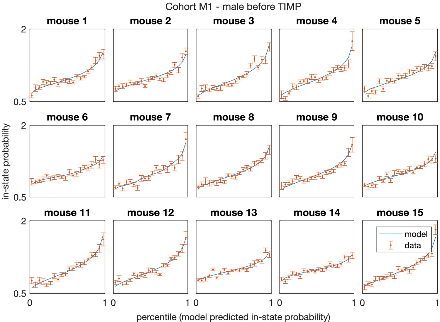
Model-predicted in-state probability matches data observation for the aggregate data of first 5 days of experiment in mice cohort M1 – C57BL/6J male mice ( $N = 15$ ), which shows the prediction of the inferred pairwise model is unbiased.

Error bars are extrapolated from 20 draws of random halves of the data.

Figure 2—figure supplement 5

Download asset Open asset

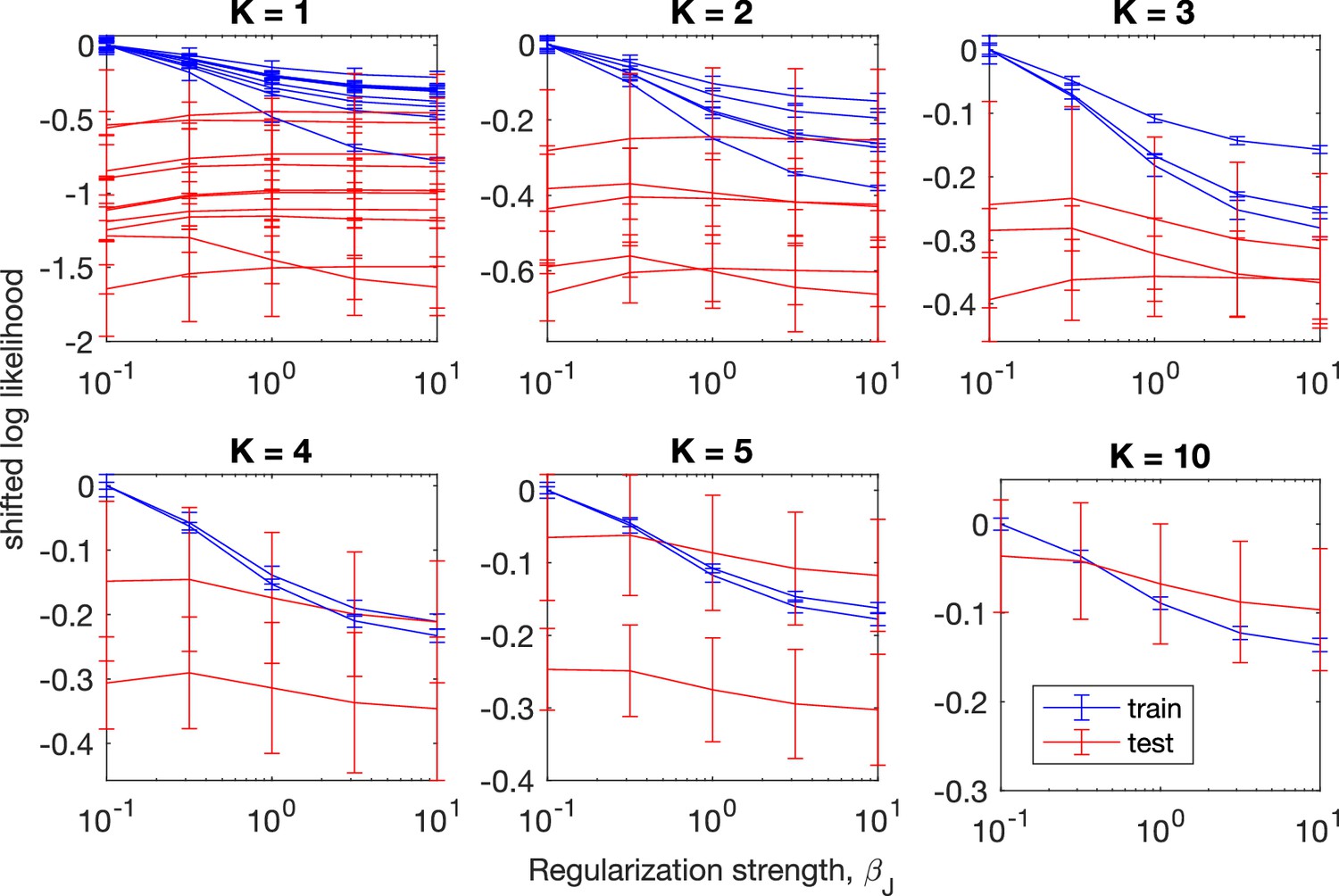
Cross-validation for maximum entropy models with triplet interactions and models with pairwise interactions on combined 10-day data (cohort M1, $N = 15$ ).

For the triplet model, L2 regularization $β_{G}$ is applied only to the triplet interactions. For the pairwise model, L2 regularization $β_{J}$ is applied only to the pairwise interactions. Error bars are standard error from the mean across six different training-test set partitions, each containing 1 hour of data as test set and 5 hours of data as training set. The maximum of test-set log likelihood is achieved when the regularization strength $β_{G}$ is large in the triplet model, and when the regularization strength $β_{J}$ is small in the pairwise model, indicating that the triplet model overfits for the data pulled from all 10 days.

Figure 2—figure supplement 6

Download asset Open asset

Cross-validation for maximum entropy models with pairwise interactions on combined data from a total of $K$ days (cohort M1, $N = 15$ ).

The plotted log-likelihoods are shifted by the training-set log likelihood at L2 regularization strength $β_{J} = 10^{- 1}$ . The L2 regularization strength $β_{J}$ is applied only to the pairwise interactions. Error bars are standard error from the mean across six different training-test set partitions, each containing 1 hour of data as test set and 5 hours of data as training set. For $K = 1$ , the test-set likelihood increases as the regularization strength $β_{J}$ increases, indicating that the pairwise maximum entropy model overfits if we only consider data from each day; while for $K \geq 4$ , the test-set likelihood decreases as the regularization parameter increases, indicating no overfitting.

Figure 2—figure supplement 7

Download asset Open asset

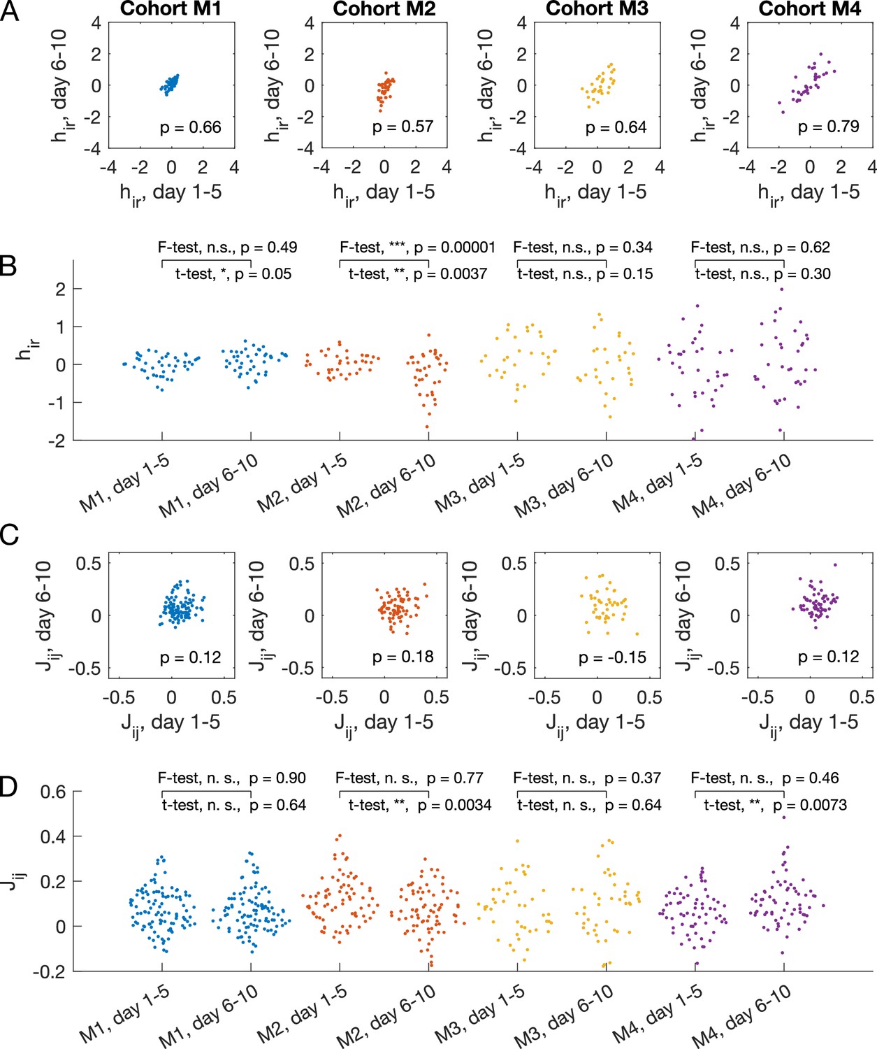
Temporal consistency of inferred parameters from 5-day accumulated data for mice cohorts M1 ( $N = 15$ ), M2 ( $N = 13$ ), M3 ( $N = 10$ ), M4( $N = 12$ ).

(A) Chamber preference for each mouse in each box, $h_{i r}$ , between models learned from the accumulated data from days 1–5, compared to the model learned from accumulated data from days 6–10. The Pearson’s correlation coefficient is shown on the plot. (B) Swarm plot for inferred pairwise interactions for each cohort from the first 5 days and the last 5 days. Two-sided t-test for equal mean and two-sided F-test for equal variance are performed. The asterisks encode the following p-values: $* p \leq 0.05; * * p \leq 0.01; * * * p \leq 0.001$ . (C) and (D) are the same as (A) and (B) for the pairwise interaction between mouse $i$ and mouse $j$ , $J_{i j}$ .

Figure 2—figure supplement 8

Download asset Open asset

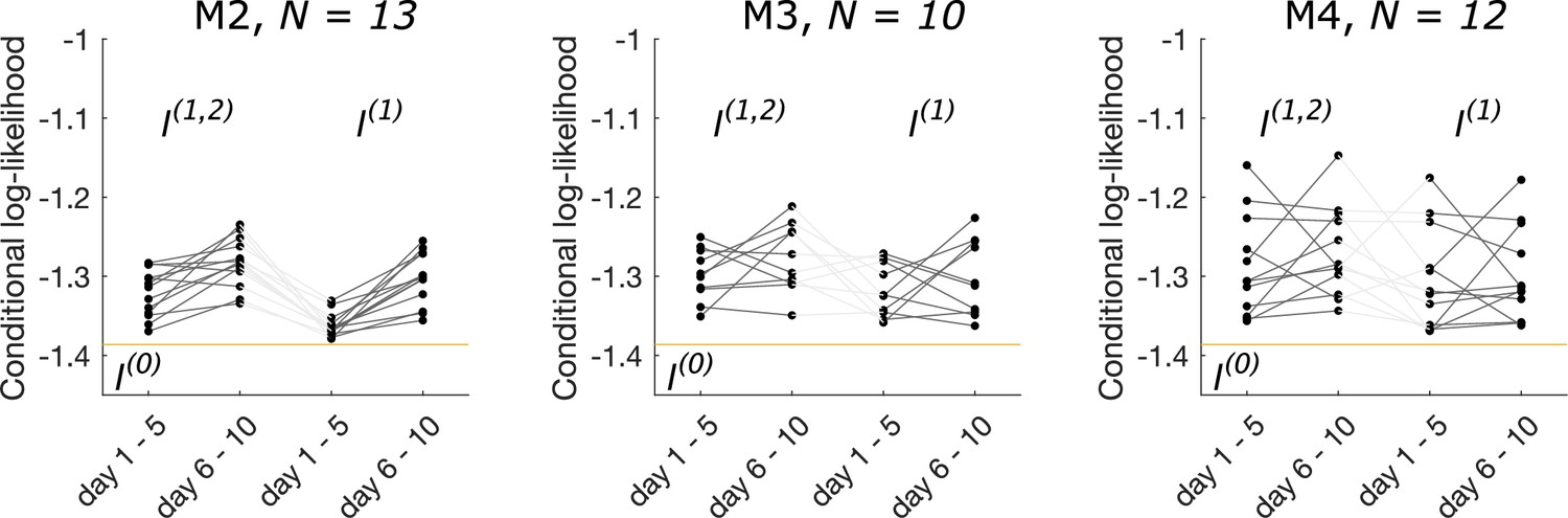
The conditional log likelihood is different for each cohort of C57BL/6J male mice $N = 13$ in cohort M2, $N = 10$ in cohort M3, and $N = 12$ in cohort M4 (before BSA injection), exhibiting individuality.

Figure 3 with 2 supplements

Download asset Open asset

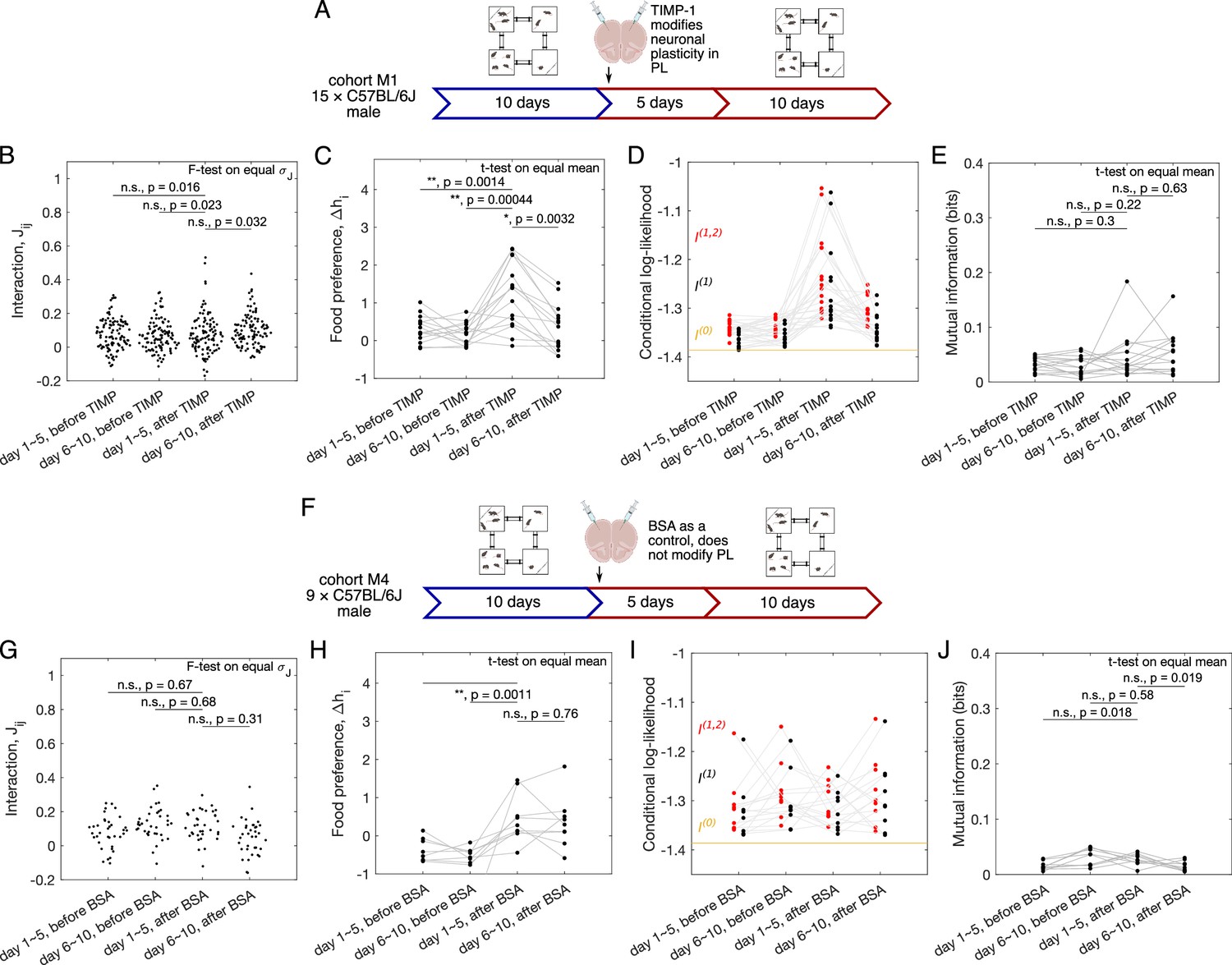
Quantification of sociability and the impact of the impaired neuronal plasticity in the prelimbic cortex (PL).

(A) Schematic of the experiment, in which neuronal plasticity in the PL of the tested subjects was impaired with TIMP-1 treatment. A cohort of C57BL/6J male mice ( $N = 15$ ) was tested in Eco-HAB for 10 days, and then removed from the cages for neuronal plasticity manipulation procedures. After a recovery period, they were placed back in Eco-HAB for another 10 days. For each of the 5-day aggregate of the experiment, both before and after TIMP-1 treatment, we plot (B) the model-inferred interactions $J_{i j}$ , (C) preference for food compartments $Δ h_{i}$ , (D) conditional log-likelihood for the pairwise model, $l^{(1, 2)}$ , the independent model, $l^{(1)}$ , and the baseline null model, $l^{(0)}$ , and (E) mutual information between single mouse position and the rest of the network given by the inferred pairwise model. (**F–J**) Same as (**A–E**), now for male C57BL/6J mice subject to injection of BSA-infused nanoparticles, a control which does not impair neuronal plasticity in the PL (cohort M4, $N = 9$ ).

Figure 3—figure supplement 1

Download asset Open asset

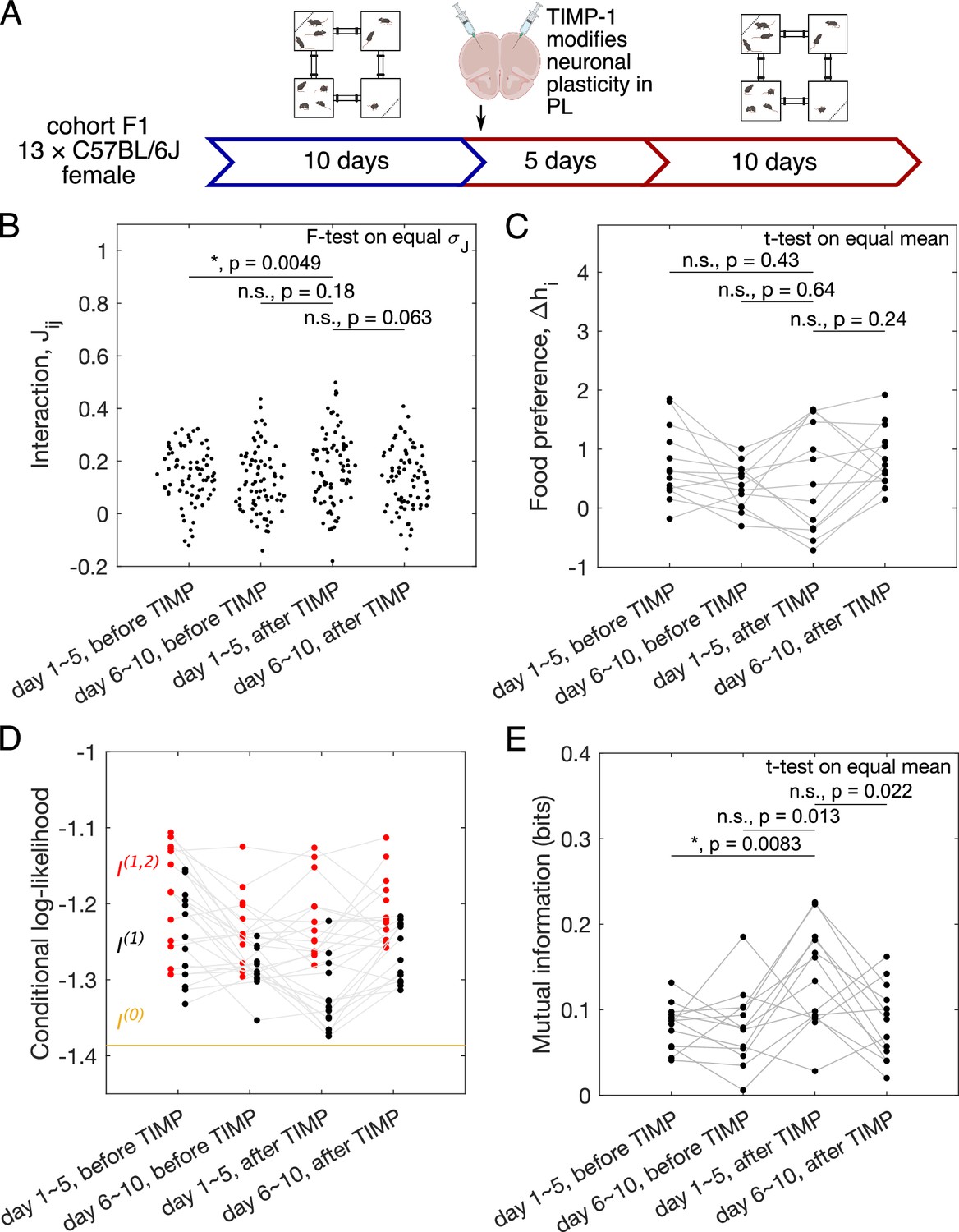
Same as Figure 3A–E, now for female C57BL/6J mice subject to injection of TIMP-1-infused nanoparticles (cohort F1, $N = 13$ ).

Figure 3—figure supplement 2

Download asset Open asset

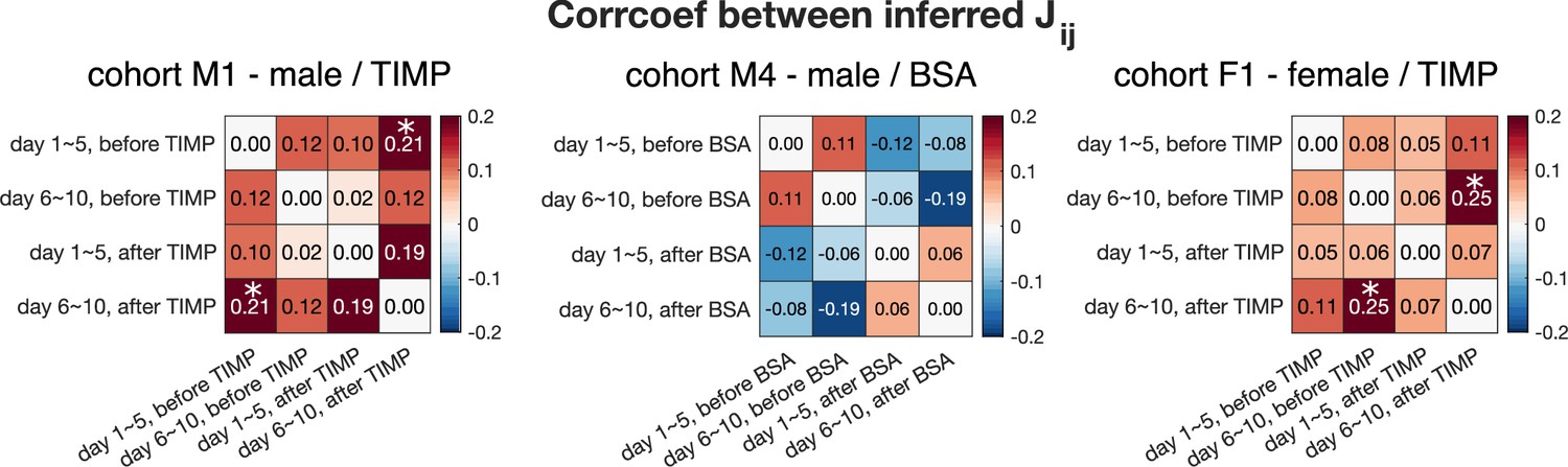
Pearson’s correlation coefficient between inferred interaction $J_{i j}$ from different 5-day aggregated data, before and after drug injection, for cohorts M1 (N = 15), M4 (N = 9), and F1 (N = 13).

Asterisks indicate statistical significance. Almost no correlation is detected between the inferred $J_{i j}$ . The only two comparisons that exhibit statistical significance are between the first and last 5 days after TIMP injection for cohort M1 (p-value=0.033), and between last 5 days before TIMP and last 5 days after TIMP injection for cohort F1 (p-value=0.028).

Figure 4 with 3 supplements

Download asset Open asset

Effect of TIMP-1 on the structure of the interaction network.

(A) Schematics of how triplets of mice may enter a state of ‘dissatisfaction’ due to competitive pairwise interactions. Dissatisfaction reduces the space of preferable states due to competitive interactions. (B) The global dissatisfaction triplet index (DTI), $F$ , computed using inferred interaction from 5-day segments of the data shows that for both male and female mice treated with TIMP-1 the global DTI is significantly increased after drug treatment, for cohorts M1 ( $N = 15$ ), M4 ( $N = 9$ ), and F1 ( $N = 13$ ). Two-sided Welch’s t-test is performed to test the significance of the difference of the global DTI between the first 5 days after drug injection against the other 5-day segments of the data. Error bars estimate the data variability, which is generated by taking random halves of the data (see ‘Materials and methods’ for details).

Figure 4—figure supplement 1

Download asset Open asset

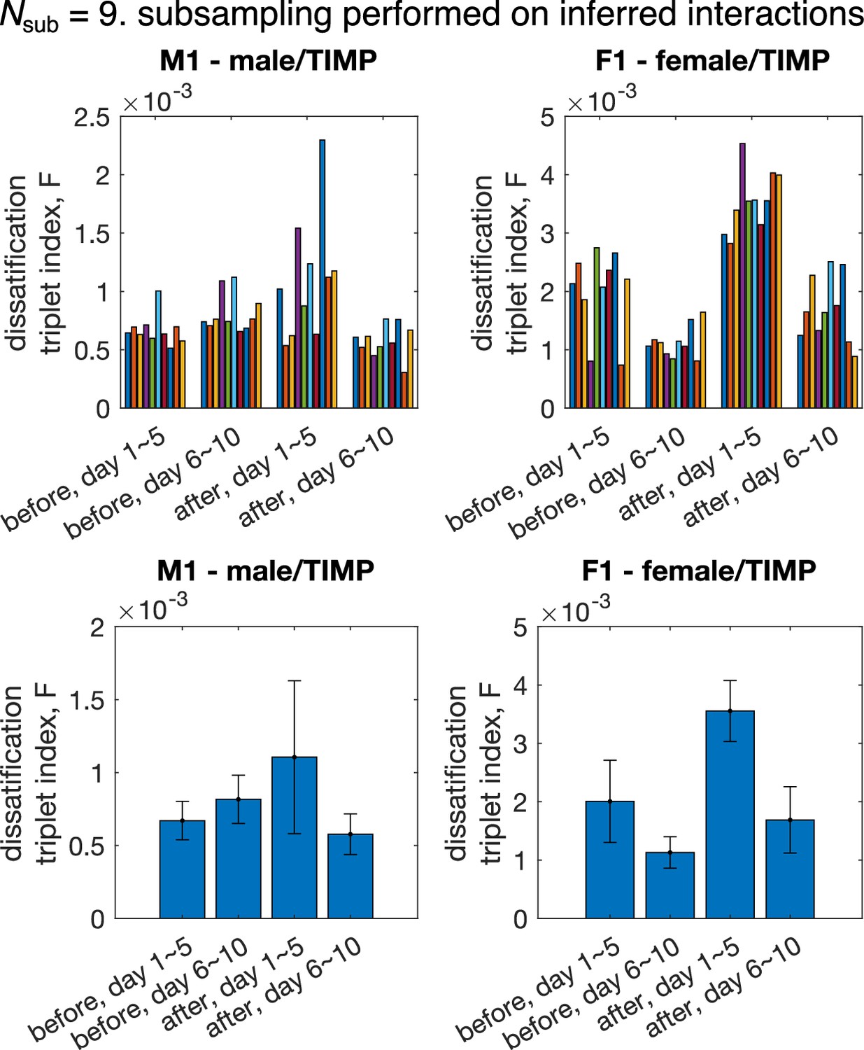
Dissatisfaction triplet index $F$ computed using subgroups of mice for cohorts M1 ( $N = 15$ , $N_{sub} = 9$ ) and F1 ( $N = 13$ , $N_{sub} = 9$ ).

Subsampling is performed at the level of inferred interactions, that is, interactions $J_{i j}$ among all $N$ mice are inferred using the pairwise maximum entropy model, then, 10 random subgroups of $N_{sub}$ mice are drawn. Top: each colored bar represent 1 realization of the subsampling. Bootstraps of random halves of the data were used in analysis to be consistent Figure 4. Bottom: average over subgroups of the bar plot in the top row. Error bar represents standard deviation across different realizations of subgroups.

Figure 4—figure supplement 2

Download asset Open asset

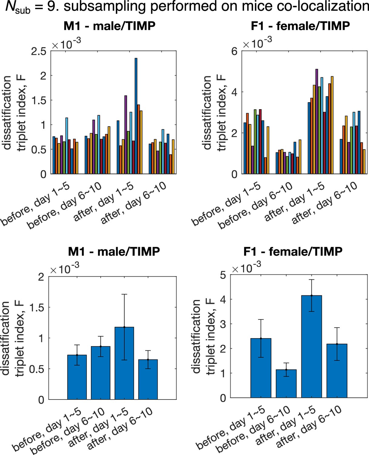
Dissatisfaction triplet index computed using subgroups of mice from cohorts M1 and F1.

Subsampling is performed at the data level, hat is, the co-localization patterns of $N_{sub}$ randomly selected mice are used to infer the interaction strengths, which are then used to compute the dissatisfaction triplet index $F$ .

Figure 4—figure supplement 3

Download asset Open asset

The global dissatisfaction triplet index (DTI) computed using shuffled interaction, $F_{shuffled}$ versus the global DTI computed using the inferred interaction, $F_{random half}$ , for cohorts M1 ( $N = 15$ ), M4 ( $N = 9$ ), and F1 ( $N = 13$ ).

Each point corresponds to one random half of the data. The two sets of global DTI’s are equal within the range of the error bars, computed by standard deviation across 20 random shuffling of the inferred interaction $J_{i j}$ , which shows the global DTI comes from the value of the inferred interaction, and that there is no additional network structure of the inferred interaction.

Tables

Table 1

Summary of experiments used in this study.

The column $N_{mice}$ gives the number of mice in the cohort used for the analysis, with cohort M4 and F1 containing dead or inactive mice after injection. The original number of mice is included in the parenthesis, and the exclusion procedure is described in ‘Exclude inactive and dead mice from analysis’. The column ‘NP’ indicates the load of the injected nanoparticles. The column ‘Day 1’ indicates the first day of observation in each of the 10-day experiment.

Cohort ID	Gender	$N_{mice}$	$T_{days}$	Day 1, WT	NP	Day 1, NP
M1	Male	15	10×2	180,511	TIMP-1	180,526
M2	Male	13	10	181,012	N/A	N/A
M3	Male	10	10	200,701	N/A	N/A
M4	Male	9 (out of 12)	10×2	200,713	BSA	200,727
F1	Female	13 (out of 14)	10×2	180,413	TIMP-1	180,430

Additional files

MDAR checklist: https://cdn.elifesciences.org/articles/94999/elife-94999-mdarchecklist1-v1.pdf
Download elife-94999-mdarchecklist1-v1.pdf

Download links

A two-part list of links to download the article, or parts of the article, in various formats.

Downloads (link to download the article as PDF)

Open citations (links to open the citations from this article in various online reference manager services)

Mendeley

Cite this article (links to download the citations from this article in formats compatible with various reference manager tools)

Xiaowen Chen
Maciej Winiarksi
Alicja Puścian
Ewelina Knapska
Thierry Mora
Aleksandra M Walczak

(2025)

Modeling collective behavior in groups of mice housed under semi-naturalistic conditions

eLife 13:RP94999.

https://doi.org/10.7554/eLife.94999.4

Share this article

Cite this article

Mice were tested in Eco-HAB, a system for automated, ecologically relevant assessment of voluntary behavior in groups of mice.

Stability of the data, given by the time evolution across 10 days of the experiment and the scatter plot between the observables measured using the first 5 days of the data versus the last 5 days of the data for cohort M1 (N=15).

Mice in Eco-HAB interact pairwisely.

The pairwise maximum entropy model reproduces the probability for each mouse in each compartment, mir, and the probability for pairs of mice in the same compartment, Cij, as given by the data.

Learned parameters in the pairwise interaction model versus the observed statistics, plotted for the 5-day aggregate data from the first 5 days of the experiment on male cohort M1 before TIMP-1 treatment.

The probability of K mice found in the same compartment, predicted by the pairwise maximum entropy model, the independent model, and computed from the 5-day aggregate data for the first 5 days in male cohort M1 before TIMP-1 treatment (N=15).

Model-predicted in-state probability matches data observation for the aggregate data of first 5 days of experiment in mice cohort M1 – C57BL/6J male mice (N=15), which shows the prediction of the inferred pairwise model is unbiased.

Cross-validation for maximum entropy models with triplet interactions and models with pairwise interactions on combined 10-day data (cohort M1, N=15).

Cross-validation for maximum entropy models with pairwise interactions on combined data from a total of K days (cohort M1, N=15).

Temporal consistency of inferred parameters from 5-day accumulated data for mice cohorts M1 (N=15), M2 (N=13), M3 (N=10), M4(N=12).

The conditional log likelihood is different for each cohort of C57BL/6J male mice N=13 in cohort M2, N=10 in cohort M3, and N=12 in cohort M4 (before BSA injection), exhibiting individuality.

Quantification of sociability and the impact of the impaired neuronal plasticity in the prelimbic cortex (PL).

Same as Figure 3A–E, now for female C57BL/6J mice subject to injection of TIMP-1-infused nanoparticles (cohort F1, N=13).

Pearson’s correlation coefficient between inferred interaction Jij from different 5-day aggregated data, before and after drug injection, for cohorts M1 (N = 15), M4 (N = 9), and F1 (N = 13).

Effect of TIMP-1 on the structure of the interaction network.

Dissatisfaction triplet index F computed using subgroups of mice for cohorts M1 (N=15, Nsub=9) and F1 (N=13, Nsub=9).

Dissatisfaction triplet index computed using subgroups of mice from cohorts M1 and F1.

The global dissatisfaction triplet index (DTI) computed using shuffled interaction, Fshuffled versus the global DTI computed using the inferred interaction, Frandom half, for cohorts M1 (N=15), M4 (N=9), and F1 (N=13).

Summary of experiments used in this study.

MDAR checklist

Downloads (link to download the article as PDF)

Open citations (links to open the citations from this article in various online reference manager services)

Cite this article (links to download the citations from this article in formats compatible with various reference manager tools)

Stability of the data, given by the time evolution across 10 days of the experiment and the scatter plot between the observables measured using the first 5 days of the data versus the last 5 days of the data for cohort M1 ( $N = 15$ ).

The pairwise maximum entropy model reproduces the probability for each mouse in each compartment, $m_{i r}$ , and the probability for pairs of mice in the same compartment, $C_{i j}$ , as given by the data.

The probability of $K$ mice found in the same compartment, predicted by the pairwise maximum entropy model, the independent model, and computed from the 5-day aggregate data for the first 5 days in male cohort M1 before TIMP-1 treatment ( $N = 15$ ).

Model-predicted in-state probability matches data observation for the aggregate data of first 5 days of experiment in mice cohort M1 – C57BL/6J male mice ( $N = 15$ ), which shows the prediction of the inferred pairwise model is unbiased.

Cross-validation for maximum entropy models with triplet interactions and models with pairwise interactions on combined 10-day data (cohort M1, $N = 15$ ).

Cross-validation for maximum entropy models with pairwise interactions on combined data from a total of $K$ days (cohort M1, $N = 15$ ).

Temporal consistency of inferred parameters from 5-day accumulated data for mice cohorts M1 ( $N = 15$ ), M2 ( $N = 13$ ), M3 ( $N = 10$ ), M4( $N = 12$ ).

The conditional log likelihood is different for each cohort of C57BL/6J male mice $N = 13$ in cohort M2, $N = 10$ in cohort M3, and $N = 12$ in cohort M4 (before BSA injection), exhibiting individuality.

Same as Figure 3A–E, now for female C57BL/6J mice subject to injection of TIMP-1-infused nanoparticles (cohort F1, $N = 13$ ).

Pearson’s correlation coefficient between inferred interaction $J_{i j}$ from different 5-day aggregated data, before and after drug injection, for cohorts M1 (N = 15), M4 (N = 9), and F1 (N = 13).

Dissatisfaction triplet index $F$ computed using subgroups of mice for cohorts M1 ( $N = 15$ , $N_{sub} = 9$ ) and F1 ( $N = 13$ , $N_{sub} = 9$ ).

The global dissatisfaction triplet index (DTI) computed using shuffled interaction, $F_{shuffled}$ versus the global DTI computed using the inferred interaction, $F_{random half}$ , for cohorts M1 ( $N = 15$ ), M4 ( $N = 9$ ), and F1 ( $N = 13$ ).