Embedding stochastic dynamics of the environment in spontaneous activity by prediction-based plasticity
- Department of Bioengineering, Imperial College London, United Kingdom
- RIKEN Center for Brain Science, RIKEN ECL Research Unit, Japan
- RIKEN Pioneering Research Institute, Japan
Figures
Figure 1
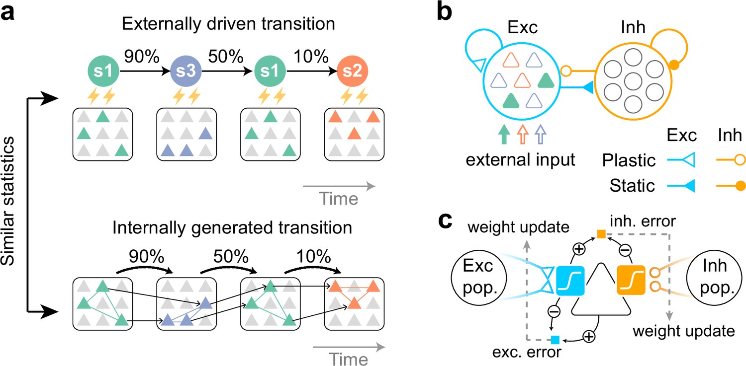
Task to be learned.
(a, top) An example of a task used to test the model. Stimulus patterns evolve in time according to structured transition probabilities. The presentation of each stimulus pattern activates the corresponding group of neurons. Recurrent connections are learned by synaptic plasticity (a, bottom). The learned network should replay assemblies spontaneously, where the transition statistics are consistent with the evoked stimuli. (b) A network model with distinct excitatory and inhibitory populations. Only excitatory populations are driven by external inputs. Only synapses that project to excitatory neurons are assumed to be plastic. (c) A schematic of the proposed plasticity rules. Excitatory (blue) and inhibitory (orange) synapses projecting to an excitatory neuron (triangle) obey different plasticity rules. For excitatory synapses, errors between internally driven excitation (blue sigmoid) and the output of the cell provide feedback to the synapses (dashed arrow) and modulate plasticity (blue square; exc. error). All excitatory connections seek to minimize these errors. For inhibitory synapses, the error between internally driven excitation (blue sigmoid) and inhibition (orange sigmoid) must be minimized to maintain excitation-inhibition balance (orange square; inh. error).
Figure 2 with 7 supplements
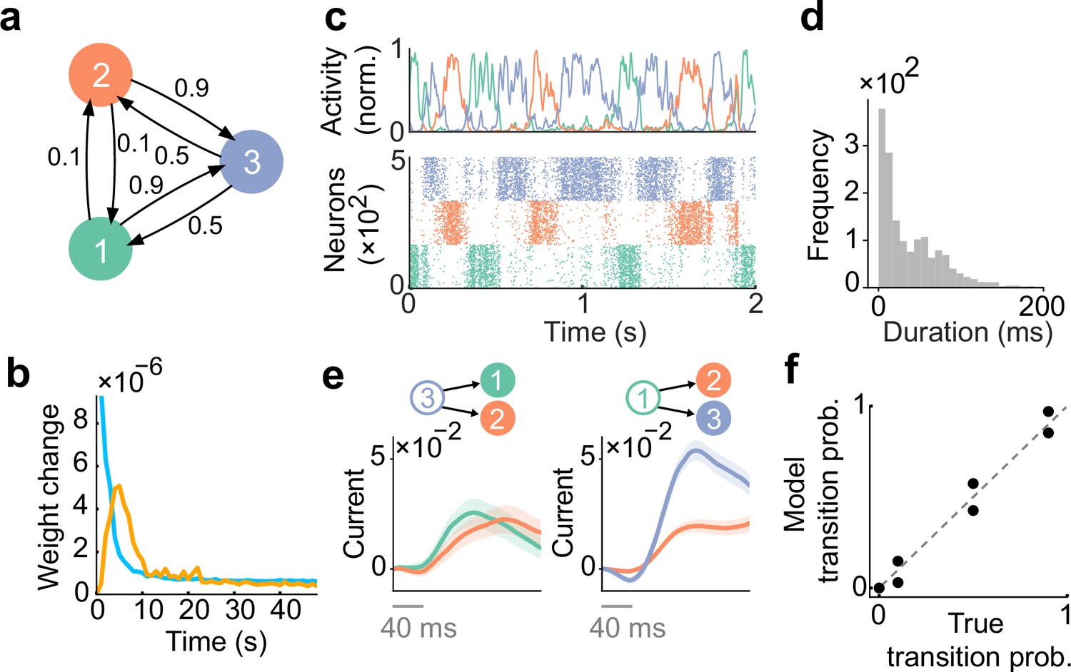
Spontaneous replay of stochastic transition of assemblies.
(a) First, we considered a simple stochastic transition between three stimulus patterns. (b) Dynamics of weight change via plasticity. Excitatory synapses (blue) converged quicker than inhibitory synapses (orange). (c) Example spontaneous assembly reactivations (top) and raster plot (bottom) of the learned network are shown. Colors indicate the corresponding stimulus patterns shown in a. (d) Distribution of assembly reactivations. (e, left) The network currents to assembly 1 (green) and assembly 2 (orange) immediately after the reactivation of assembly 3 ceased. Both currents were similar in magnitude. (e, right) Currents to assembly 2 (orange) and assembly 3 (blue) immediately after the reactivation of assembly 1 ceased. The current to assembly 3 was stronger than that to assembly 2. (f) Relationship between the transition statistics of stimulus patterns and that of replayed assemblies. The spontaneous activity reproduced transition statistics of external stimulus patterns.
Figure 2—figure supplement 1
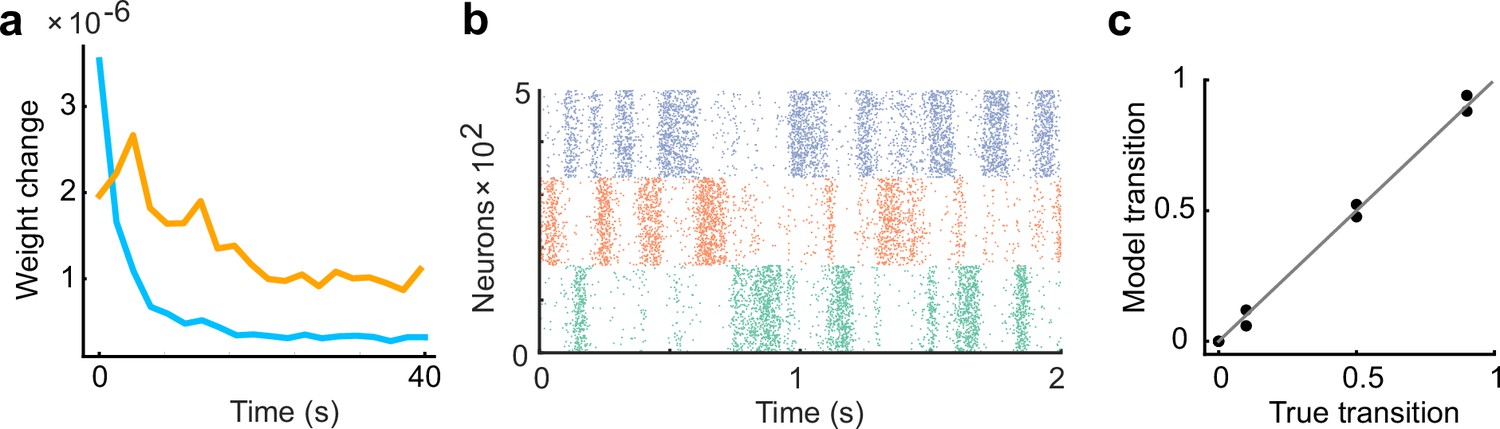
Inhibitory plasticity lags behind excitatory plasticity.
(a) The learning rate of inhibitory plasticity was made twice that of excitatory plasticity. The inhibitory plasticity still occurred on a slower timescale than excitatory plasticity (Froemke et al., 2007). (b) Example raster plot of spontaneous assembly reactivations of the learned network are shown. (c) Even if the learning rate of inhibitory plasticity was larger, the spontaneous activity reproduced transition statistics of external stimulus patterns.
Figure 2—figure supplement 2

Unstructured spontaneous activity before learning.
Example spontaneous assembly reactivations (top) and raster plot (bottom) of the network are shown. Colors indicate the corresponding stimulus patterns shown in Figure 2a.
Figure 2—figure supplement 3

The network performance is less sensitive to the duration of evoked assembly activations during learning.
(a) The distributions of the durations of the assembly reactivations after training with input states of half the duration of the initial setting are shown. (b) The spontaneous activity of the trained network still showed appropriate transition dynamics.
Figure 2—figure supplement 4
The network performance dependence on cell assembly size.
(a) The network was trained with the assembly size ratio of 1:1.5:2. (b) In the case of a, the spontaneous activity after training reproduced an appropriate transition statistics. (c) The network was trained with the assembly size ratio of 1:2:3. (d) In the case of c, the network showed less performance.
Figure 2—figure supplement 5
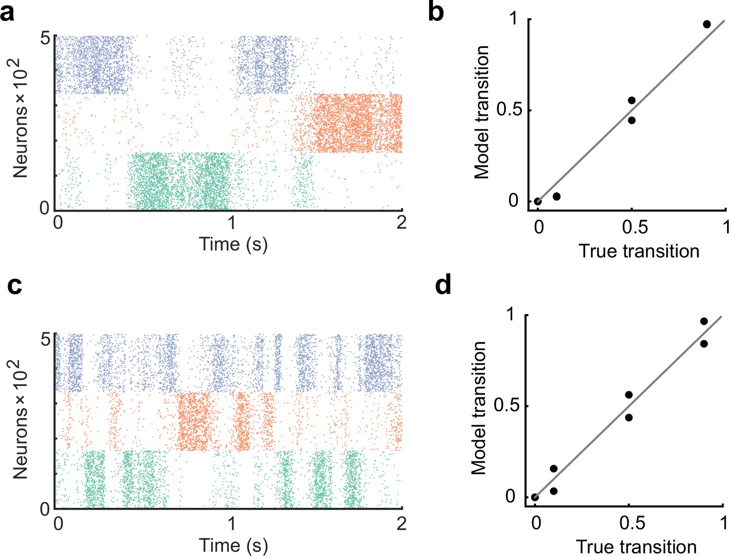
The learning rate controls the duration of cell assembly reactivations.
(a) The learning rate of all plasticity was made half that of the original settings in Figure 2. (b) In the case of a, the spontaneous activity reproduced the transition statistics of the external stimulus patterns. (c) The learning rate of all plasticity was made twice that of the original settings in Figure 2. The duration of assembly reactivations was shorter than in a. (d) Spontaneous activity reproduced transition statistics of external stimulus patterns.
Figure 2—figure supplement 6
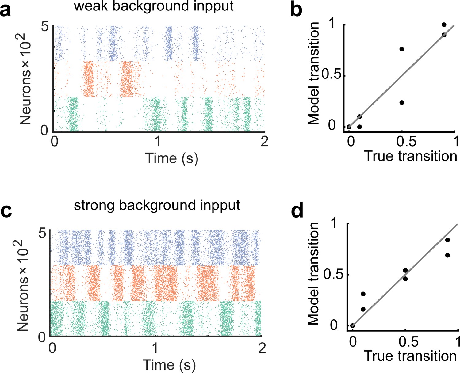
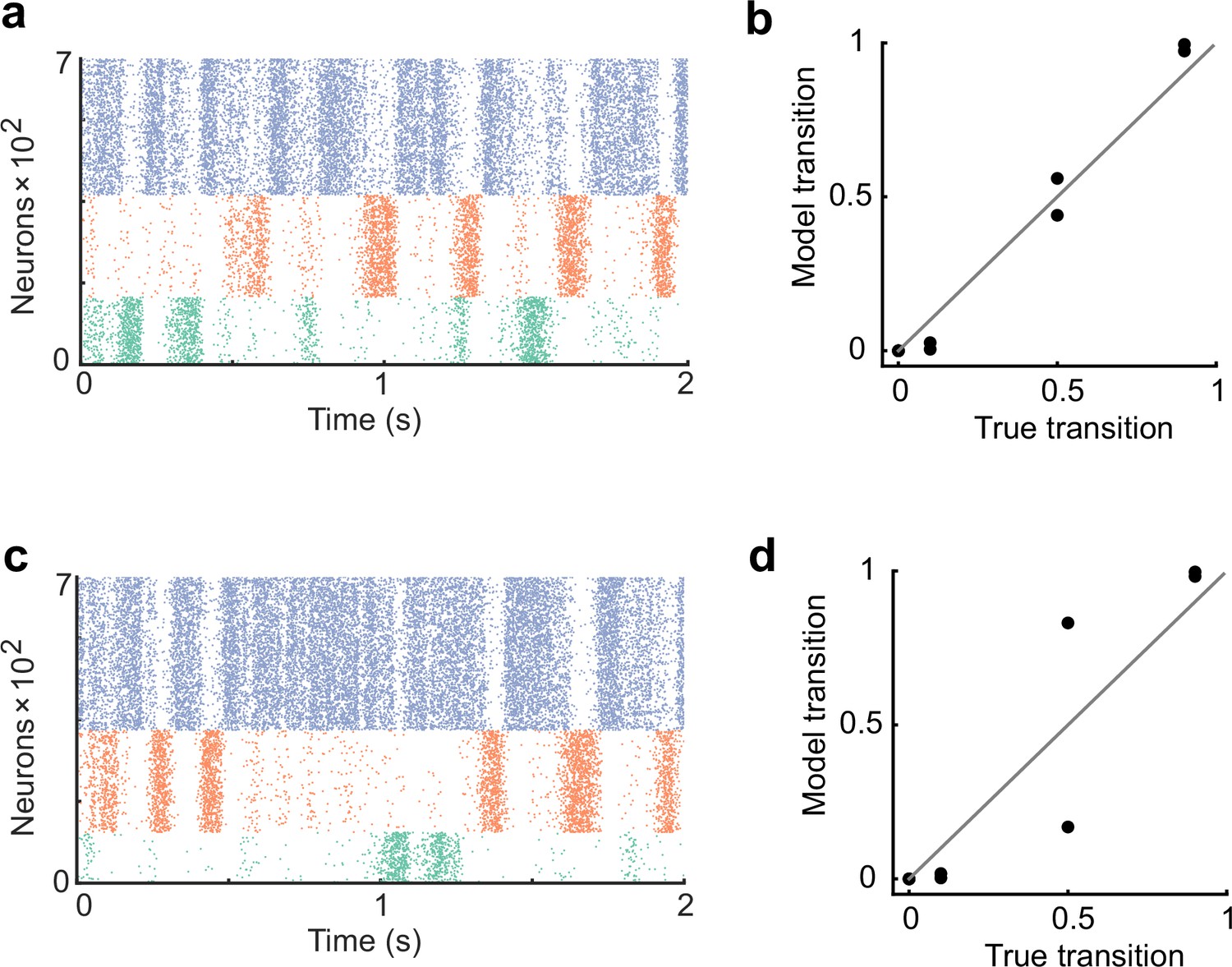
The network performance dependence on the strength of background input.
(a) The network was trained and tested with half the strength of the background input compared to the case in Figure 2. (b) The network showed worse performance than the case shown in Figure 2. (c) The network was trained and tested with double the strength of the background input compared to the case in Figure 2. (d) The network exhibited more uniform transitions compared to the case in Figure 2.
Figure 2—figure supplement 7
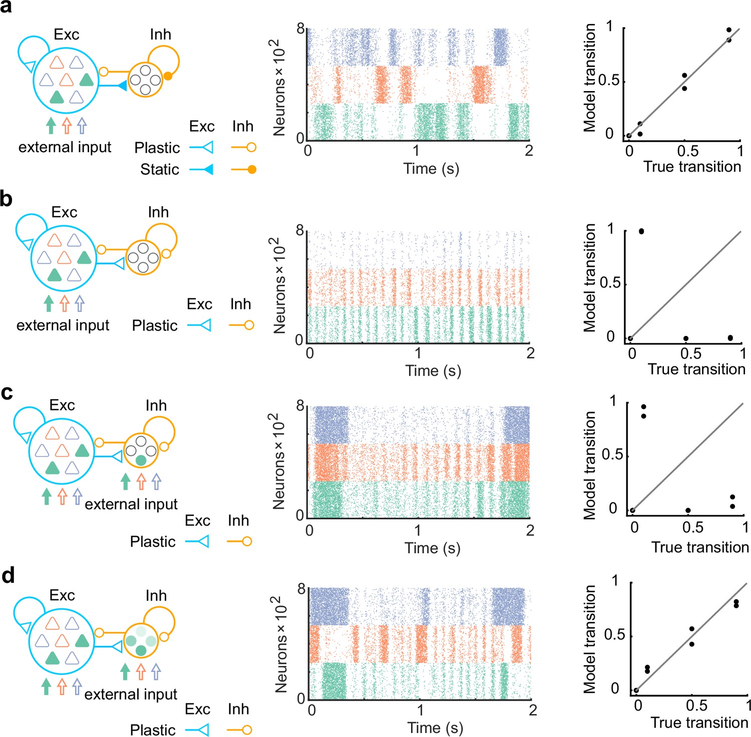
The networks with more biologically plausible architectures.
(a) The network consists of 80% of excitatory neurons and 20% of inhibitory neurons was trained. Same as in Figure 1, synapses projecting on excitatory neurons only were trained (left). The network after training showed spontaneous activity with appropriate transition statistics (middle, bottom). (b) Same with a, but all synapses were assumed to be plastic. The network spontaneous activity did not show appropriate transitions. (c) Same with b, but all network neurons receive the external input. The network spontaneous activity did not show appropriate transitions. (d) Same with c, but all inhibitory neurons had mixed selectivity. Here, we assumed that when each state is presented, all inhibitory neurons are driven with a randomly assigned intensity between 0 and 2. The spontaneous activity showed appropriate transitions in this case.
Figure 3 with 2 supplements
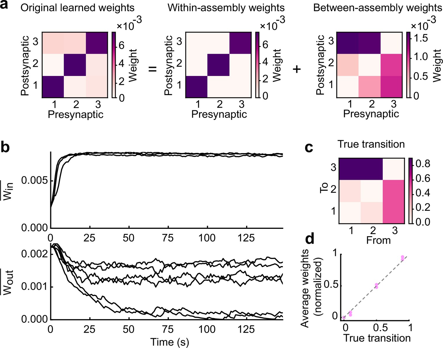
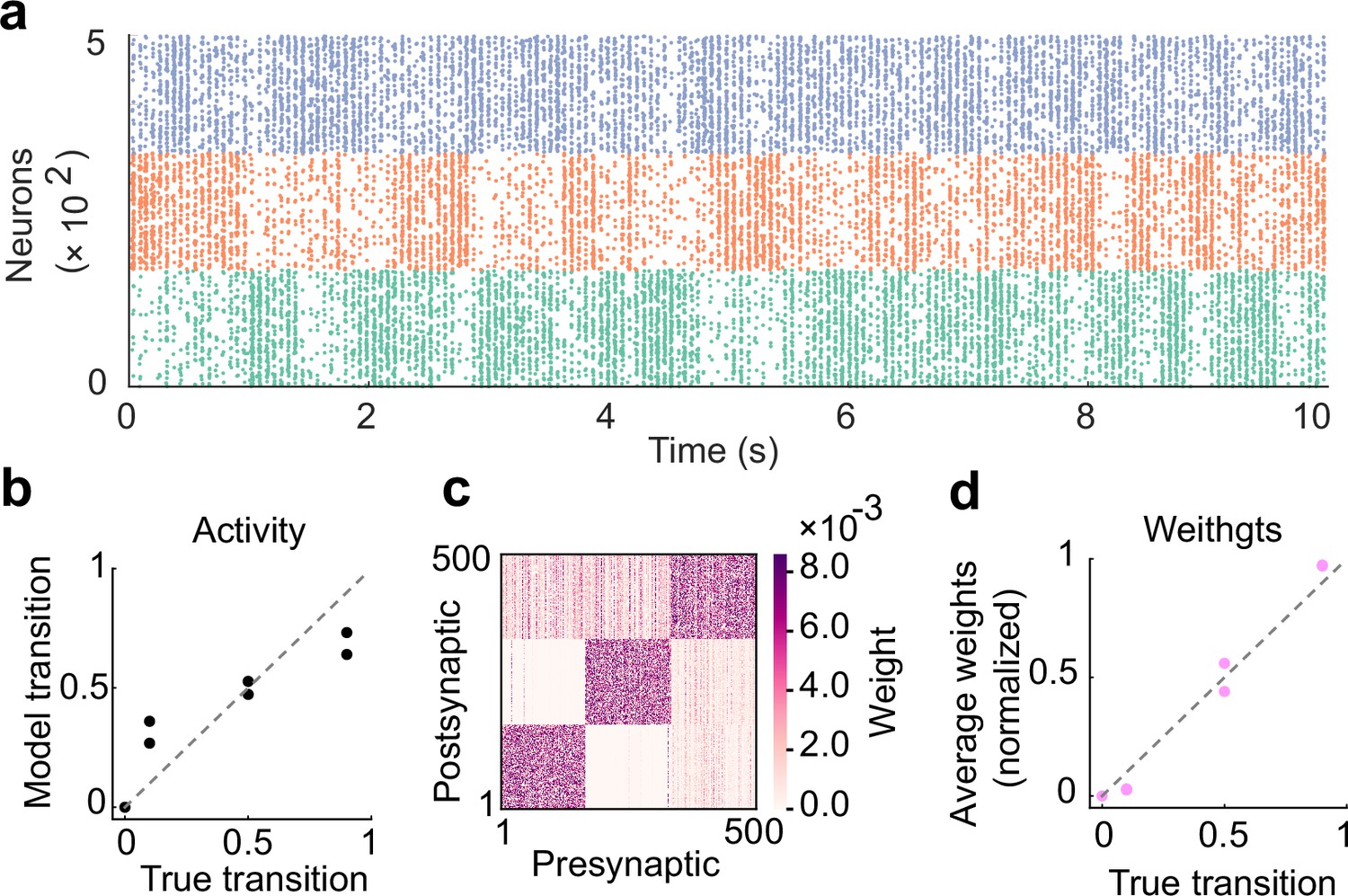
Learned excitatory synapses encode transition statistics.
(a) A 3 by 3 matrix of excitatory connections, learned with the task in Fig.2a (left). The matrix can be decomposed to within- (middle) and between-assembly connections (right). (b) Strength of within- (top) and that of between-assembly excitatory synapses (bottom) during learning are shown. (c) True transition matrix of stimulus patterns. (d) Relationship between the strength of excitatory synapses between assemblies and true transition probabilities between patterns.
Figure 3—figure supplement 1
The role of inhibitory plasticity in transition probability learning.
(a) Example spontaneous assembly of a model without inhibitory plasticity is shown. (b) Relationship between the transition statistics of stimulus patterns and that of replayed assemblies. (c) Learned excitatory weights. (d) Relationship between the strength of excitatory synapses between assemblies and true transition probabilities between patterns.
Figure 3—figure supplement 2
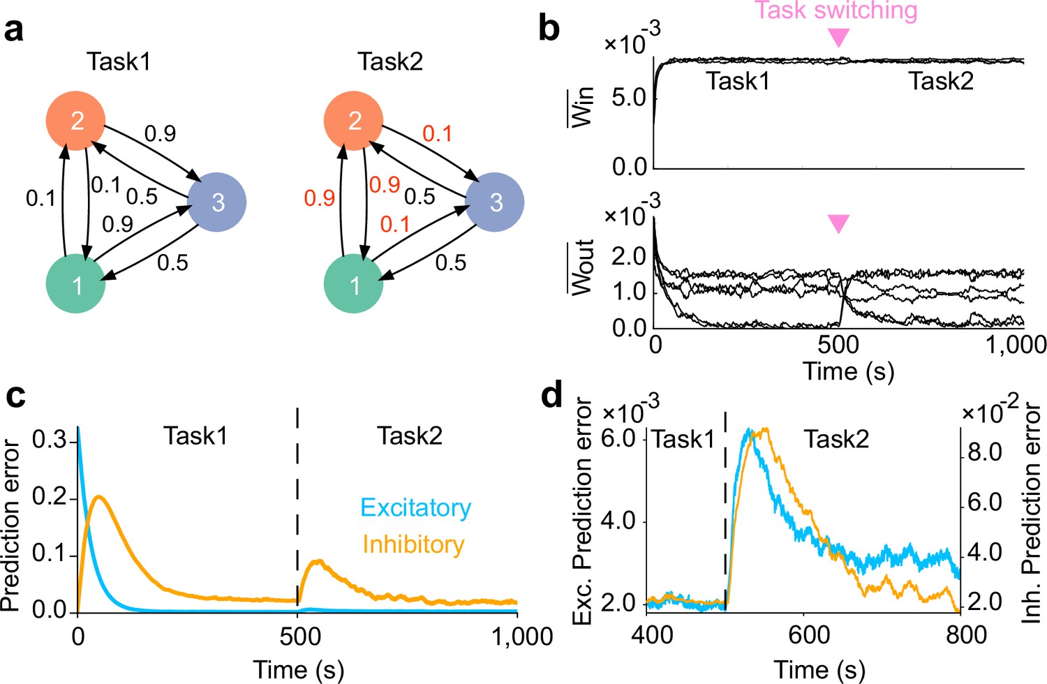
Network adaptation to task switching.
(a) Two types of tasks were considered. (b) Strength of within- (top) and that of between-assembly excitatory synapses (bottom) during learning are shown. Switching from task1 to task2 was occured at the middle of learning phase (inverted triangles). Between-assembly connectivity reorganized once the task switching occurred. (c) Dynamics of prediction error for excitatory (blue) and inhibitory (orange) plasticity are shown. (d) Magnified versions of c are shown. Both errors show an abrupt increase immediately after task switching, followed by a gradual decay. In c and d, errors were calculated as averages over five independent simulations.
Figure 4 with 2 supplements
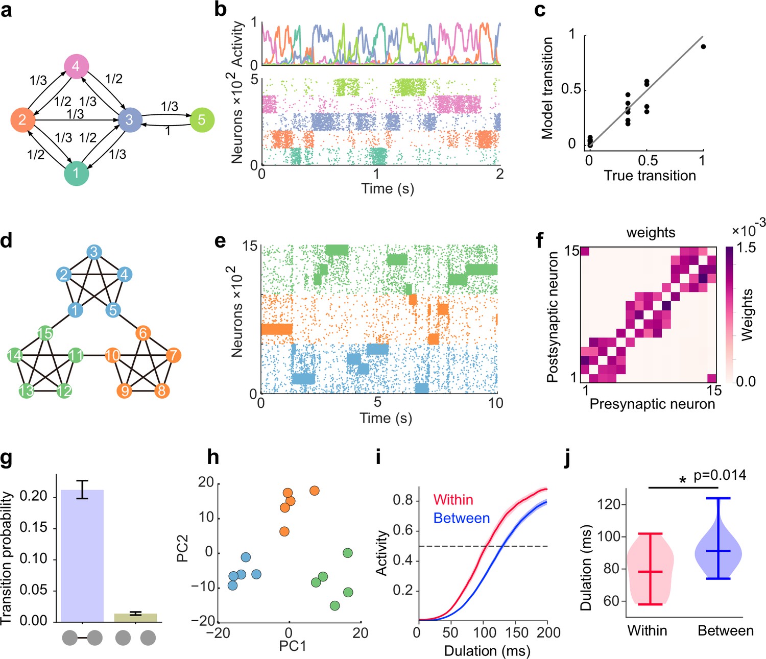
Learning complex structures.
(a) Transition diagram of complex task. (b) Spontaneous activity of learned network. (c) Transition statistics of assemblies reproduce true statistics. (d) Transition diagram of temporal community structure. (e) Raster plot of spontaneous activity of the network trained over structure shown in (d). (f) Structure of learned excitatory synapses encode the community structure. (g) Spontaneous transition between assemblies connected in the diagram shown in d occurs much frequent than disconnected case. (h) Low dimensional representation of evoked activity patterns shows high similarity with community structure. (i) Time courses of replayed activities transitioning within (red) and between (blue) communities. (j) Comparison of mean durations in (i). P-value was calculated by two-sided Welch’s t-test.
Figure 4—figure supplement 1

The excitatory synapses learned transition structures of complex task shown in Figure 4a.
Figure 4—figure supplement 2
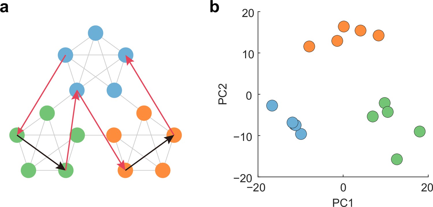
Low-dimensional community structure reflects learned weights, not input order.
(a) Scrambled structure in which presentation rule of patterns violates temporal community structure. Scrambled sequence consists of both learned (black arrows) and untrained (red arrows) transitions, which viorates the community structure. The network underwent scrambled task only after it learned community structure shown in Figure 4d. (b) Low-dimensional representation of activity patterns evoked by scrambled sequence.
Figure 5
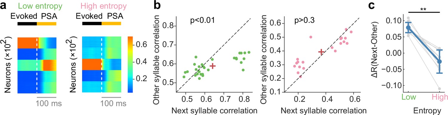
Network dynamics consistent with recorded neural data of songbird.
(a) Example poststimulus activity (PSA) for low- (left) and high-entropy (right) transition cases. (b) Comparison of correlation coefficients between PSA and evoked single-syllable responses for next syllables and other syllables. For low entropy transition case, the next-syllables correlations were significantly higher than other-syllables correlations (p < 0.01, Wilcoxon signed-rank test) (left). In contrast, such correlation coefficients showed no significant difference for high entropy transition case (p > 0.3, Wilcoxon signed-rank test) (right). Red crosses are mean. (c) The difference in correlation coefficients between next and other syllables (ΔR) was significantly greater for low entropy transitions than for high entropy transitions (p < 0.01, two-sided Welch’ s t-test).
Tables
Table 1
Definition of variables and functions.
| , | Membrane potentials |
|---|---|
| , | Postsynaptic potentials |
| Poisson spike train generated by network neurons | |
| , , , | Recurrent connections |
| External current elicited by stimulus presentation | |
| Synaptic currents generated by network neurons | |
| , | Instantaneous firing rates |
| , | Recurrent predictions |
| Memory trace | |
| Dynamic sigmoidal function | |
| Static sigmoidal function | |
| , | Filtered prediction errors |
Table 2
Parameter settings.
| Connection probability | 0.5 | |
|---|---|---|
| Gain parameter in sigmoid function | 2 | |
| , | Network size | 500, 500 (1500,1500 in Figure 5e-j; 800, 200 in Figure 2—figure supplement 7) |
| Learning rate | 10-4 | |
| Synaptic time constant | 5 ms | |
| Membrane time constant | 15 ms | |
| , | Parameters for sigmoid | 5, 1 |
| Time constant of memory trace | 10 s | |
| Maximal firing rate | 50 Hz | |
| Scaling factor of synaptic current | 25 | |
| Time constant for low-pass filtering the error | 30 s | |
| Constant external current during spontaneous activity | 0.3 |
Additional files
Download links
A two-part list of links to download the article, or parts of the article, in various formats.
Downloads (link to download the article as PDF)
Open citations (links to open the citations from this article in various online reference manager services)
Cite this article (links to download the citations from this article in formats compatible with various reference manager tools)
Embedding stochastic dynamics of the environment in spontaneous activity by prediction-based plasticity
eLife 13:RP95243.
https://doi.org/10.7554/eLife.95243.3


