Figures and data in CausalXtract, a flexible pipeline to extract causal effects from live-cell time-lapse imaging data | eLife

Figures
Videos
Additional files

3 figures, 3 videos and 1 additional file

Figures

Figure 1 with 1 supplement

Download asset Open asset

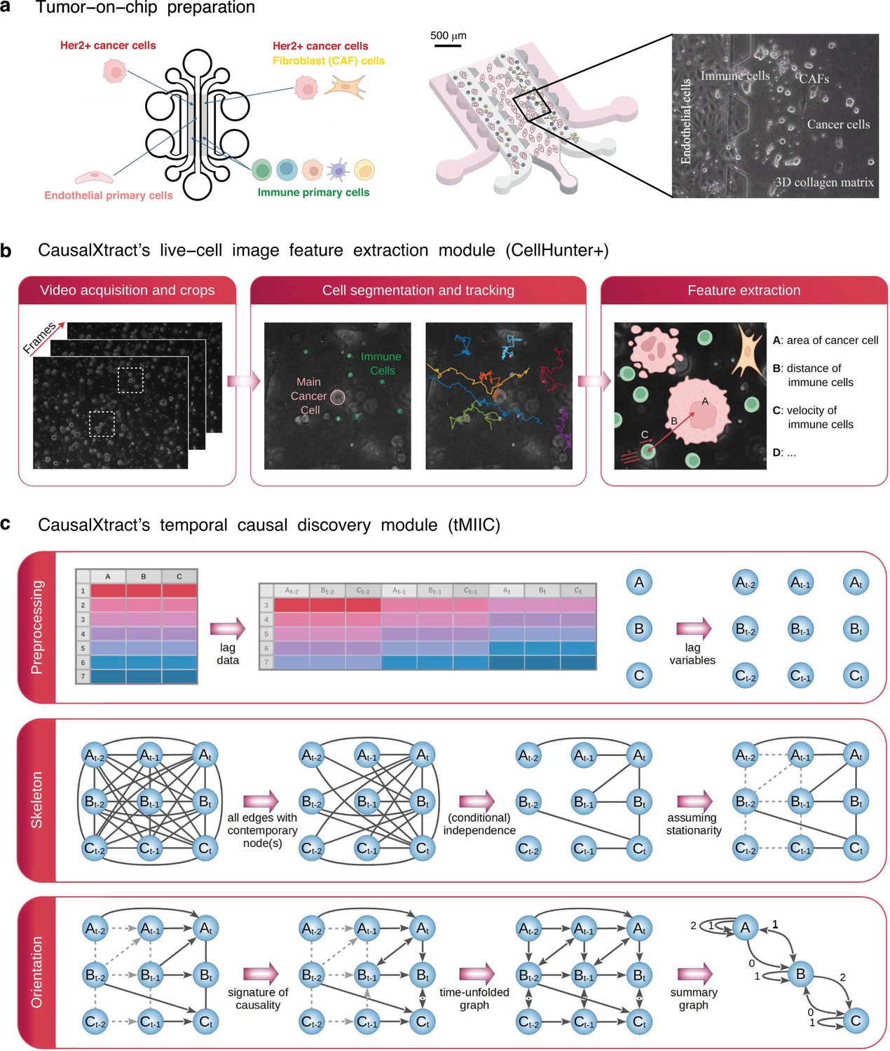
CausalXtract pipeline.

(a) Live-cell tumor ecosystem reconstituted ex vivo (Nguyen et al., 2018) using the tumor-on-chip technology (‘Materials and methods’). (b) CausalXtract’s live-cell image feature extraction module (CellHunter+). The tracking of cancer and immune cells and of their mutual interactions is illustrated in Videos 1–3, in the absence or presence of cell division and apoptosis event. Examples of time series of extracted cellular features are shown in Figure 1—figure supplement 1. (c) CausalXtract’s temporal causal discovery module (tMIIC) learns a temporal causal network from the features extracted in (b). See ‘Materials and methods’ for CausalXtract’s implementation details and theoretical foundations. A step-by-step notebook of CausalXtract pipeline is provided with the source code.

Figure 1—figure supplement 1

Download asset Open asset

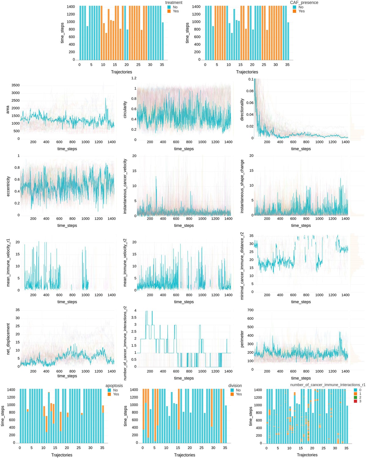
Time series of cellular features extracted from the tumor ecosystems.

Example of time series of cellular features extracted by CausalXtract’s feature extraction module (CellHunter+) from the tumor ecosystems analyzed in this study (Figure 1a). It includes two experimental control parameters (i.e., treatment and CAF presence) and 15 cellular features extracted every 2 min over a period of 2 days. Continuous features are highlighted for one trajectory (traj.18), while categorical features are shown for all trajectories.

Figure 2 with 4 supplements

Download asset Open asset

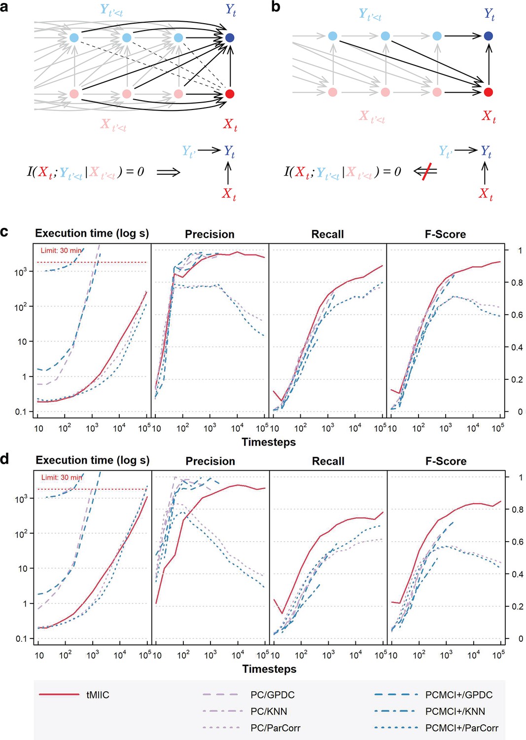
Relation to Granger–Schreiber temporal causality and tMIIC benchmarking against PC and PCMCI+.

(a) The signature of Granger–Schreiber temporal causality is a vanishing Transfer Entropy, that is, $T_{Y \to X} = I (X_{t}; Y_{t^{'} < t} | X_{t^{'} < t}) = 0$ (‘Materials and methods’). In the time-unfolded causal network framework, it implies (i) the absence of (dashed) edge between $X_{t}$ and any $Y_{t^{'}}$ , with $t^{'} < t$ , and (ii) if $X_{t}$ is adjacent to $Y_{t}$ , the presence of temporal (2-variable+time) v-structures, $Y_{t^{'}} \to Y_{t} \leftarrow X_{t}$ , for all $Y_{t^{'}}$ adjacent to $Y_{t}$ , with $t^{'} < t$ (‘Materials and methods’, Theorem 1). (b) By contrast, the presence of a temporal (2-variable+time) v-structure, $Y_{t^{'}} \to Y_{t} \leftarrow X_{t}$ does not imply a vanishing Transfer Entropy as long as there remains an edge between any $Y_{t^{''} < t}$ and $X_{t}$ . It implies that Granger–Schreiber temporal causality is in fact too restrictive and may overlook actual causal effects, which can be uncovered by graph-based causal discovery methods. Hence, tMIIC’s time-unfolded network framework, combining graph-based and information-based approaches, sheds light on the common foundations of the seemingly unrelated graph-based causality and Granger–Schreiber temporal causality, while clarifying their actual differences and limitations. (c) Benchmarking of tMIIC on synthetic time-series datasets generated from 15-node causal networks based on linear combinations of contributions, Appendix 1 and Figure 2—figure supplements 1–3. (d) Benchmarking with more complex 15-node time-series datasets based on nonlinear combinations of contributions, Appendix 2 and Figure 2—figure supplement 4. Running times and scores (Precision, Recall, Fscore) are averaged over 10 datasets and compared to PC and PCMCI+ methods using different kernels (GPDC, KNN, ParCorr).

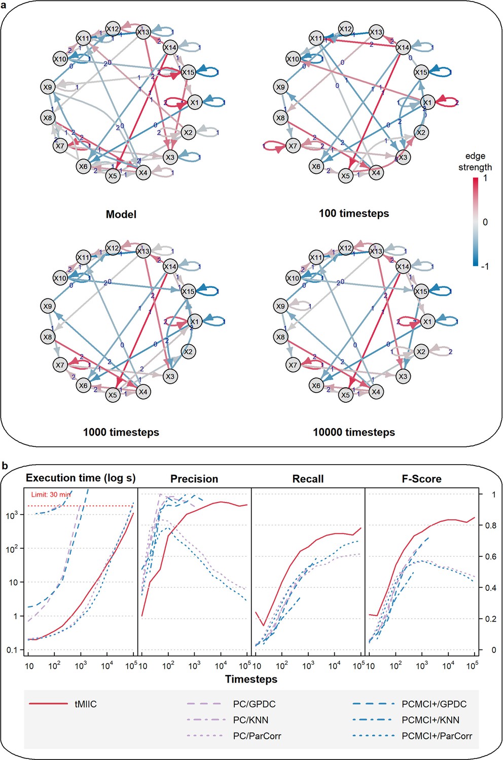
Figure 2—figure supplement 1

Download asset Open asset

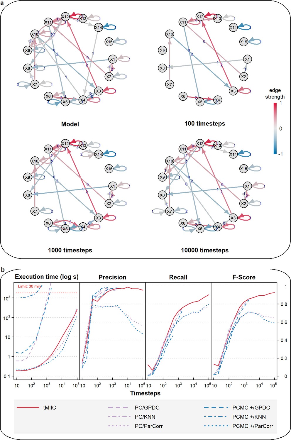
Benchmark assessment of CausalXtract’s causal discovery module (tMIIC) using generated time-series datasets.

(a) Example of a 15-node causal network to generate benchmark time-series datasets based on linear combinations of contributions (Appendix 1). Examples of temporal causal networks reconstructed by tMIIC based on 100, 1000, or 10,000 simulated time steps. (b) Running times and scores (Precision, Recall, Fscore) averaged over 10 datasets and compared to PC and PCMCI+ methods using different kernels (GPDC, KNN, ParCorr); tMIIC is at par with PC and PCMCI+ scores using GPDC and KNN kernels but runs orders of magnitude faster. Only ParCorr kernel matches tMIIC running speed but with significantly lower scores at large sample size; see ‘Materials and methods’.

Figure 2—figure supplement 2

Download asset Open asset

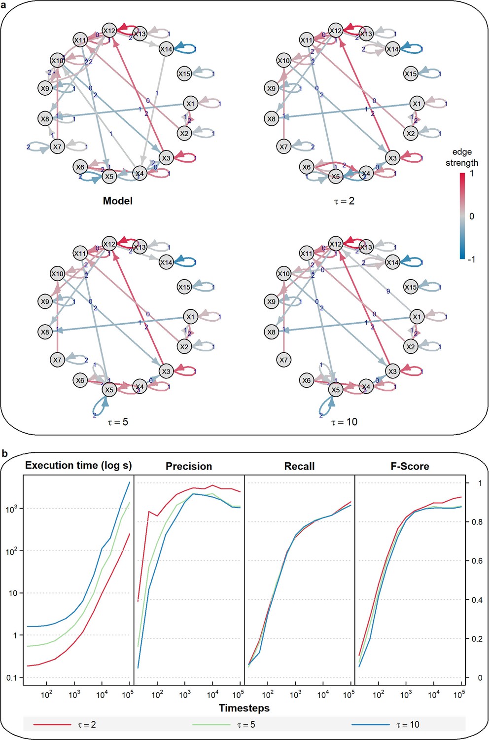
CausalXtract insensitivity to an overestimated maximum lag τ.

Figure 2—figure supplement 3

Download asset Open asset

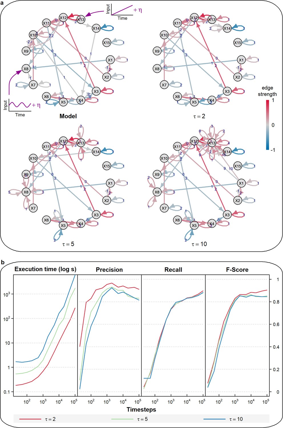
CausalXtract sensitivity to non-stationary variables.

(a) Example of a temporal causal network model ( $τ = 2$ ) with a low-frequency periodic input ( $T = 100$ ) applied to X8 and a time-linear trend applied to X13. Corresponding temporal causal networks inferred by tMIIC from 1000 time step time series (Appendix 1) including non-stationary inputs to X8 and X13. Increasing the maximum lag from $τ = 2$ to $τ = 5$ or 10 leads to the appearance of multiple self-loops, which result from the non-stationary dynamics of X8 and X13, whilst the rest of the network remains largely unaffected. (b) Running times and scores (Precision, Recall, Fscore ignoring X8 and X13 self-loops) of tMIIC causal network reconstructions for $τ = 2, 5$ or 10 averaged over 10 time series of 10 to 10⁵ time steps.

Figure 2—figure supplement 4

Download asset Open asset

Benchmark assessment of CausalXtract’s causal discovery module (tMIIC) using more complex time-series datasets.

(a) Example of a 15-node causal network to generate more complex benchmark time-series datasets based on nonlinear combinations of contributions (Appendix 2). Examples of temporal causal networks reconstructed by tMIIC based on 100, 1000, or 10,000 simulated time steps. (b) Running times and scores (Precision, Recall, Fscore) averaged over 10 datasets and compared to PC and PCMCI+ methods using different kernels (GPDC, KNN, ParCorr); tMIIC outperforms both PC and PCMCI+, in terms of Recall and Fscores, while running orders of magnitude faster, except for the ParCorr kernel, which leads, however, to significantly lower scores at large sample size.

Figure 3 with 2 supplements

Download asset Open asset

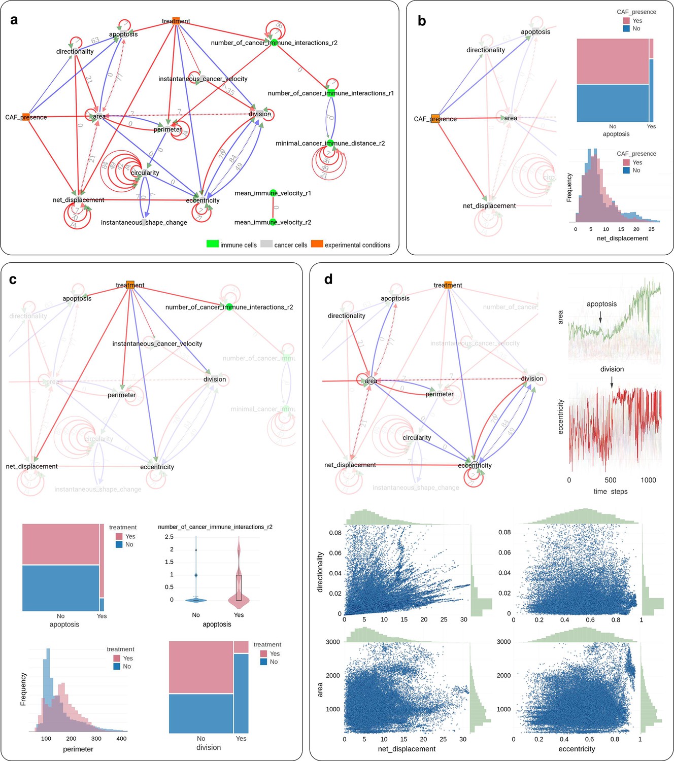
Application of CausalXtract to time-lapse images of tumor ecosystems reconstituted ex vivo.

(a) Summary causal network inferred by CausalXtract. The underlying time-unfolded causal network is shown in Figure 3—figure supplement 1. Red (resp. blue) edges correspond to positive (resp. negative) associations. Bidirected dashed edges represent the effect of unobserved (latent) common causes. Annotations on edges correspond to time delays in time steps (1 ts = 2 min). The inferred network is largely robust to variations in sampling rate ( $δ τ$ ) and maximum lag ( $τ$ ), Figure 3—figure supplement 2. Here, $δ τ = 7$ ts and $τ = 84$ ts are chosen automatically by CausalXtract. (b) The CAF presence subnetwork highlighting the direct causal effects of CAFs on cancer cells. In particular, CausalXtract uncovers that CAFs directly inhibit cancer cell apoptosis independently from treatment, which has not been reported so far. (c) The treatment subnetwork highlighting the direct causal effects of treatment on cancer cells. In particular, CausalXtract uncovers that treatment increases cancer cell perimeter, which has not been reported either. (d) The eccentricity-area subnetwork highlighting multiple direct and possibly antagonistic time-lagged effects, notably, between cell division and eccentricity and between cell apoptosis and area, as discussed in the main text.

Figure 3—figure supplement 1

Download asset Open asset

Time-unfolded causal network inferred by CausalXtract.

(a) Time-unfolded causal network assuming stationary dynamics of cellular ecosystems implying translational time invariance of the inferred causal network. (b) Only edges involving at least one contemporaneous variables (i.e., at time t) need to be tested for conditional independence by tMIIC and the remaining edges are then duplicated at all previous time steps before assigning orientations when time-lagged latent variables are taken into account (Figure 1c). Variables retaining multiple self-loops with different time delays correspond to non-stationary variables in Figure 1—figure supplement 1, in agreement with benchmarks from simulated data including non-stationary variables (Figure 2—figure supplement 3).

Figure 3—figure supplement 2

Download asset Open asset

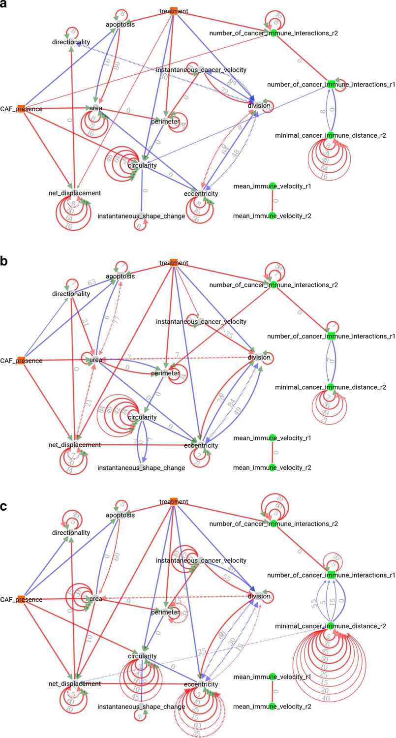
Robustness of CausalXtract’s temporal causal networks to variations in sampling rate.

Summary causal networks inferred by CausalXtract using different sampling rates ( $δ τ$ ). (a) $δ τ = 8$ ts and $τ = 80$ ts, in time step units (1 ts = 2 min). (b) $δ τ = 7$ ts, and $τ = 84$ ts, as chosen automatically by CausalXtract based on the average relaxation time across the 15 monitored variables, $τ_{R} = 40$ ts, which defines a maximum lag $τ = 2 τ_{R} = 80$ ts. Given a total number of (time-lagged and -unlagged) nodes, chosen to be around 200 nodes for computational efficiency, it leads to 13 temporal layers ( $ν + 1 = 200 / 15 ≃ 13$ ) and a lag increment $δ τ = τ / ν ≃ 7$ ts. This summary causal network corresponds to Figure 3a. (c) $δ τ = 5$ ts and $τ = 60$ ts, corresponding to $τ = ν \cdot δ τ$ with $ν + 1 = 13$ temporal layers, as in (b).

Videos

Video 1

Download asset

posterframe for video — Example of tracking of cancer and immune cells and of their mutual interactions in the absence of cell division and apoptosis event.

Video 2

Download asset

posterframe for video — Example of tracking of cancer and immune cells and of their mutual interactions in the presence of a cell division event.

Video 3

Download asset

posterframe for video — Example of tracking of cancer and immune cells and of their mutual interactions in the presence of a cell apoptosis event.

Additional files

MDAR checklist: https://cdn.elifesciences.org/articles/95485/elife-95485-mdarchecklist1-v1.pdf
Download elife-95485-mdarchecklist1-v1.pdf

Download links

A two-part list of links to download the article, or parts of the article, in various formats.

Downloads (link to download the article as PDF)

Open citations (links to open the citations from this article in various online reference manager services)

Mendeley

Cite this article (links to download the citations from this article in formats compatible with various reference manager tools)

Franck Simon
Maria Colomba Comes
Tiziana Tocci
Louise Dupuis
Vincent Cabeli
Nikita Lagrange
Arianna Mencattini
Maria Carla Parrini
Eugenio Martinelli
Herve Isambert

(2025)

CausalXtract, a flexible pipeline to extract causal effects from live-cell time-lapse imaging data

eLife 13:RP95485.

https://doi.org/10.7554/eLife.95485.3

Sign up for email alerts

Privacy notice