Shortcutting from self-motion signals reveals a cognitive map in mice
Figures
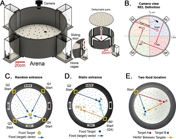
Hidden Food Maze and experimental setup.
(A) The floor of the arena is 120 cm in diameter, and the walls are 45 cm tall. Note 20 cm scale bar in this panel. The home cage has a 10.5x6.5 cm2 floor area. The door slides upward (mice enter without handling). The floor is washed and rotated between every trial to avoid predictable scratch marks and odor trails. The subfloor containing food is not illustrated. (B) Camera view of a mouse searching for hidden food (target, pointed by the target vector). The REL of the target is marked for each entrance (from the mouse’s perspective, the displacement from the start in each quadrant to its respective REL is the same for any entrance; e.g. ‘70cm forward +30 cm to the left’; and it is equal to the displacement from the trained start to target). (C) ‘Random entrances’ experiment. Mice enter from any of the four entrances randomly over trials to search for food (‘A’-labeled star) always in front of the X landmark. Arrows show the four possible displacements. (D) ‘Static entrances’ experiment. Mice start from the same entrance (labeled ‘Start’) in every trial to search for food in front of the same landmark. Blue/cyan arrows = food vector (start→food); Orange arrow = REL vector (start→REL). After training, the start position in a probe trial can be rotated (‘180o Start’) to check whether mice follow idiothetic (start→REL; ignoring landmarks) or allothetic (start→A; following landmarks) cues; going via the REL vector is regarded as evidence of path integration. (E) ‘Two food location’ experiment. Mice start from a static entrance to search for food (red vector to target A). Afterwards, mice are trained to find food in a different location (blue vector to target B). After learning both targets, a probe trial (i.e. a trial without food) is designed to check whether mice can compute shortcuts from B to A (B-A vector, orange arrow).
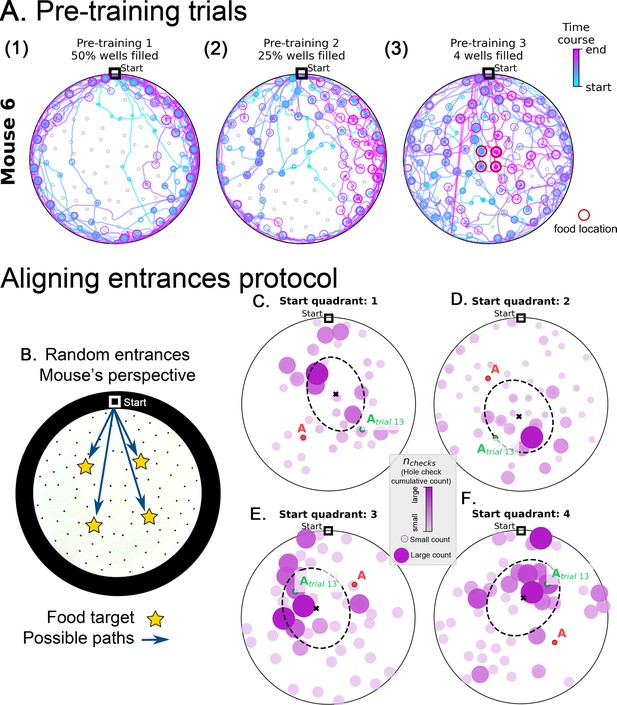
Pre-training trajectories and active sensing from the mouse perspective in random entrance experiment.
(A) Example trajectories of a mouse during pretraining (see Materials and methods). The mice are habituated to their home cage (Day 1) and the maze (Day 2, no food). On Day 3, mice start exploring an arena with randomly selected 50% of the holes filled with food (panel A1). On Day 4 25% of the holes are filled with food (panel A2). Most trajectories are confined near the maze walls on Days 3 and 4. During the final pre-training Day 5, only the four central wells (panel A3, red circles) have food and the mice now explored the entire maze. Circles indicate hole checks (with or without food) with color and size indicating the time course of checking – small, blue circles occur early along the trajectory and pink large circles later in the trajectory. Food locations are only illustrated for Day 5 where they are confined to four central holes. The mice can re-enter their home cage at any time during the food search resulting in multiple blue and magenta lines converging at the Start location. (B-F). Active sensing from the mouse perspective in random entrance experiment. B. The mouse can enter the arena from each of the four quadrants of the circle. Due to the circular symmetry, we can rotate each entrance setup so that it always aligns to the top of the screen, as shown. This is the mouse perspective of the experiment, where now the mouse has to find one of four possible target locations. (C–F) show the hole checks of trial 14 of the Random Entrance experiment as an example (target = red ‘A’ label). The previous spots of the target are shown with a green ‘Atrial 13’ label and depend on the specific entrance a particular mouse took in trial 13. Quadrants are defined in main Figure 1. Starting from Quadrant 1 is linked to the configuration in panel C; quadrant 2 in panel D; quadrant 3 in panel E; and quadrant 4 in panel F. Moreover, notice that the configuration of targets for panel D is rotated 90°Clockwise relative to panel C; panel E is 180°Clockwise relative to C; and F is 270°Clockwise relative to panel C. Thus, we can reverse these rotations and align all panels to the configuration in C (see Experiment alignment in Materials and methods). We do that consistently for every trial, increasing the sample for the active sensing at each trial. The data shown in panels C to F refer to the frequency of hole checks in the arena: number of checks accumulated over mice divided by total number of checks, normalized between zero (smaller circles colored in light pink) and one (larger circles colored in dark pink). Larger balls represent higher normalized check rates.
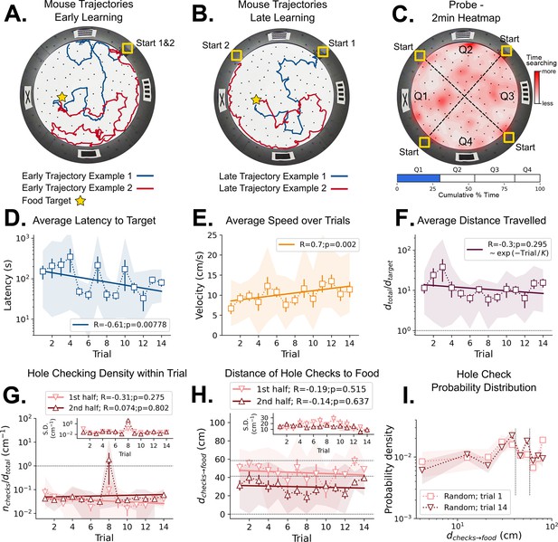
Mouse spatial learning with random entrances.
(A) Two examples of mouse search trajectories during early learning (trial 3) when the entrance changes from trial to trial. They are irregular and vary unpredictably across trials. (A, B) Star = target location. Yellow Square = entrance site. (B) Two examples of mouse search trajectories during late learning (trial 14) after starting from different entrances. Trajectories look as irregular as in early trials. (C) Top: Heatmap of the first 2 min of a probe trial done after trial 18 (red = more time in a given region). Bottom: Mice spent about the same time (25%) in each of the four sectors, regardless of being close to the target (blue) or to its REL (white). (D) Some significant reduction in latency to reach target is seen across trials (p=0.008; N=8). (D–I) Error bars = S.E. Shaded area = data range. (E) Some significant increase in speed is seen (p=0.002; N=8). (F) Average normalized distance traveled to reach target (dtotal/dtarget=1 is optimal; p=0.05, N=8). (G) Hole-checking density (number of hole checks per distance traveled) in each half of the trajectory. The density remains constant for both halves and across trials, suggesting that mice remained uncertain as to the food location. G-inset. The S.D. of the density over the mice sample remains constant for both halves (N=8). (H) The average distance of the checked holes to the food d(checks→food) remains almost constant across trials. Horizontal lines are just guides to the eye. (I) The probability density of the distance of hole checks to the food d(checks→food) for the first and last learning trials (the corresponding averages over trials are in panel H). The density remains unaltered. Vertical dotted lines mark the same distances as the horizontal lines in panel (H).
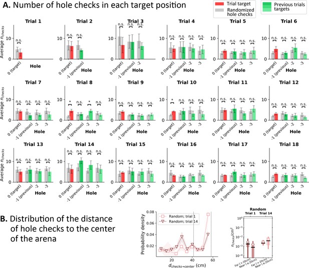
Hole check distribution in Random Entrance protocol for the four target holes from the mouse’s perspective.
(A) Red bar: hole checks in the target hole (labeled ‘0’). Green shaded bars: hole checks in the previous positions of the target in the mouse’s perspective (see Figure 1—figure supplement 1B; ‘–1’ for the position of the target in the previous trial; ‘–2’ for the trial before previous; and ‘–3’ for the trial before ‘–2’). Since, there are training trials, each of the target holes (0,–1, –2, and –3) had food in their respective trial (i.e. ‘0’ has food in the trial; –1 had food in the previous trial; –2 had food in the trial before previous; and –3 had food in the trial before –2). Gray bars: randomized hole checks for each corresponding position: all detected hole checks in a given trial were uniformly distributed across the 100 holes of the arena, and then we counted the number of checks in each of the four targets’ positions. Whiskers: standard deviation (n=8). Gray bars were compared to the corresponding colored bars via a paired t-test. Significant differences were rarely found (Trial 8 only) between randomized data and actual hole checks, suggesting that the mice are performing randomly. n.s.=not significant. (B) Left: Distribution of the distance of the hole checks to the center of the arena (to be compared with Figure 2I and Figure 3I in the main text). The distance of the active sensing to the center of the arena is almost uniform, indicating that the mice have no preferential distance to check for food. Right: The density of checks near the center (<20 cm away) is the same as farther away. This suggests that there is no obvious spatial learning feature relating the target with the central spot of the maze.
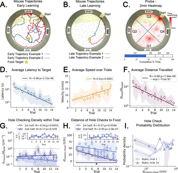
Mouse spatial learning with static entrances.
(A) Two examples of mouse search trajectories during early learning (trial 3). They are irregular and variable similarly to those in the random entrance experiments. (A, B) Star = target location. Yellow Square = entrance site. (B) Two examples of mouse search trajectories during late learning (trial 14). They go directly towards the food or go along the wall before turning to the food, creating variation across mice and trials. (C) (Top) Heatmap of the first 2 min of a probe trial done after trial 14 (red = more time in a given region). (Bottom) Mice spent almost 50% of the time within 15 cm radius of the target (blue) compared to the RELs (white). (D) Latency dramatically decreases (p<10–7; N=8). (D–I) Error bars = S.E. Shaded area = data range. (E) Speed significantly increases during trials (p=0.0001; N=8). (F) Normalized distance to reach target d(total→target)=1 is optimal becomes almost optimal (p<10–7; N=8). (G) Hole-checking density over distance in each half of the trajectory. It significantly decreases in the first half (p=0.05), and stays constant in the second. G-inset: The S.D. of the density is larger in the second half. (H) The average distance of the checked holes to the food d(checks→food) decreases for both halves of the trajectory. After learning, the hole checks happen closer to the food d(checks→food) is almost zero, although there are more checks per distance. (I) The probability density of the distance of hole checks to the food d(checks→food) for the first and last trials (the corresponding averages over trials are in panel H). After learning (trial 14), the density is larger closer to the food, a feature that does not appear in the random entrance experiments.
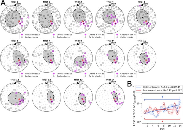
Location of hole checks in the last 3 s before finding the target in Static Entrance protocol.
(A) Pink spots: hole checks in the last 3 s before finding the target; gray spots: earlier hole checks. Dashed ellipsis (x=mean): dispersion (covariance) of the spatial distribution of hole checks. The distribution of hole checks migrates towards the target (labeled A) as the mice learn. All mice (n=8) pooled together. (B) Density of hole checks ( per traveled distance) in the last 3 s (pink spots), compared with that density for the earlier path (gray spots), as a function of trial. There is significant increase over trials (R=0.7, p=0.00545) for the static entrance case, implying that the hole checks are converging to be temporally ‘close’ to the food as the mice learn – in the first few trials, holes are checked throughout the entire duration of the run. We hypothesize that the pink spots might act as anchors for place fields. Shade behind the curve marks the full extent of the sample (n=8 mice). Stars: significant difference between first and last trial (paired t-test, p<0.05).
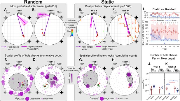
Trajectory directionality and active sensing for random and static experiments.
Arenas on the top row (mean displacement vector – see color scale between panels B and E) correspond to the ones immediately below them (hole checking spatial distribution); the red ‘A’ label marks the target (food site), which is pointed by the food (target) vector (purple arrow). Top row (A, B, E, F): the color and arrows indicate the most probable route taken (red = more probable; only p<0.001 displacements shown; pink arrow = inferred target position, or TEV; shaded pink sector = S.D. of TEV; see Materials and methods, and Figure 6—figure supplement 1). Bottom row (C, D, G, H): spatial distribution of hole-checks; size and color of circles = normalized frequency that a hole was checked (larger pink circles = higher frequency); Black ellipse (x=mean): covariance of spatial distribution. Green ellipse (+=mean): covariance of spatial distribution restricted to ≤20 cm of the target. Random entrance experiments (N=8; panels A, C: trial 1; B, D: trial 14): regardless of training stage, no significant preferred routes and the TEV does not point to target (A, B); hole checks are randomly distributed throughout the arena, and shift from the walls (C) to near the center (D) after learning. Static entrance experiments (N=8; panels E, G: trial 1; F, H: trial 14): after learning (F) the TEV and significant displacements go straight to the target (although individual trajectories are variable); and hole checks align along the start-target path (H). (I) Deviation between the TEV (pink arrow) and the target vector (purple arrow) illustrated in top panels. Directionality is quickly learned (static case). (J, K) Hole-check area density corresponding to the spatial profiles in bottom panels. Density after learning is larger near the target (static case), supporting the path integration hypothesis. Asterisks/star: p<0.05 (paired t-test). Note the presence of more significant displacements in late learning for static entrances only, and the associated alignment of the TEV and food vector.
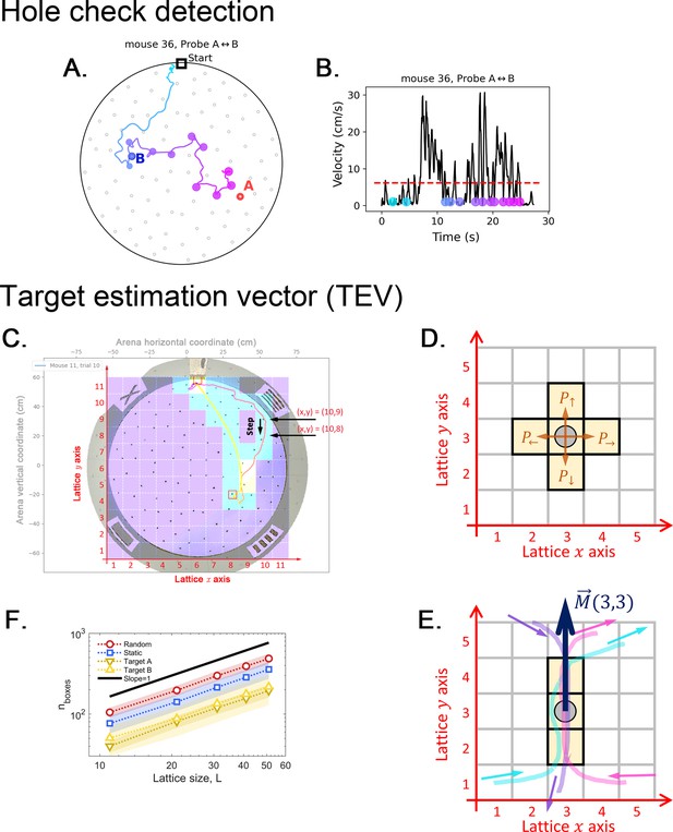
Definition of a hole-checking event as active sensing and target estimation vector (TEV).
(A) Observed trajectory with hole-checking events identified by the two criteria sets of our method, applied subsequently to avoid missed checks. (B) The velocity profile with dots representing the hole-checking events shown in panel A. The color from cyan to magenta represents the time order of the events, as presented in panel A. See Hole-checking Event detection in Materials and methods for details of the detection criteria. A video is also available at https://bit.ly/mouseCogMapVideo to illustrate the operation of the hole check algorithm and the mouse behavior. (C-E): Arena lattice, box size scaling and step map definition. (C) A square lattice with boxes is overlayed on top of the arena recording to build the step map. There are boxes along both the and axes. is an odd number, such that the center box is aligned with the center of the arena. For , each lattice site (box) measures approximately 11 cm by 11 cm. This lattice is used to calculate the step maps (see Step map calculation in Materials and methods). (D) To generate the step maps, we start by counting the number of steps a mouse takes between any two adjacent sites in the lattice; for example, when the mouse lies in the box marked by the gray circle, it can choose to take a step up, down, left or right. If no trajectories pass over that site towards a given direction, then that particular direction is assumed to have null probability . (E) An example showing three trajectories that eventually pass by the marked spot, two times going up (cyan and magenta) and one time going down. The step map vector is then pointing up. See Materials and methods for the detailed calculation of this vector. (F) We count the number of boxes for each trajectory (exemplified in panel A) and plot it versus the lattice lateral size , yielding the box dimension1 equal 1 for all trajectories in every trial and experimental setup. The observed robust scaling allows us to use moderately small for our experimental analysis; thus, larger yields qualitatively the same results.
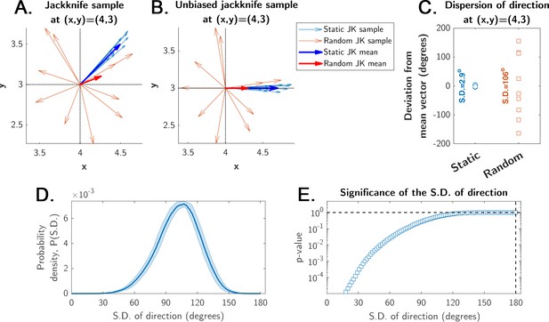
Estimation of significance for the mean displacement direction calculation.
The jackknife sampling procedure is obtained by the ‘leave-one-out’ rule, yielding N unique jackknife samples of N-1 points from an original sample of N points (see Materials and methods). (A) Illustration of a jackknife sample with N-1=10 vectors for a single site in the arena for both static (blue, strong directionality) and random (red, weak directionality due to a more uniform direction distribution) entrance experiments (pale-colored arrows = sample; bold-colored arrows = mean; the means make up the displacement maps shown in main Figures 4, 5, 7 and 8, and Figure 6—figure supplement 1). (B) The same sample from panel A, but all vectors’ angles (i.e. directions) were shifted such that the mean angle of each condition (static and random entrances) is zero degrees. This procedure does not change the distribution of angles, but makes all angles distributed with zero mean between –180o and 180o. (C) The angles of the mean displacement vectors of a typical site in the static experiment are narrowly distributed around 0o (S.D.=2.9o for this particular site, after the unbiasing in panel B); the angles of the random entrance experiments are widely distributed (S.D.=106o for this particular site), reflecting weak directionality. (D) The probability density of observing some particular value for the S.D. of a collection of N=8 uniformly distributed angles between –180o and 180o. It was calculated numerically (shaded area is the error of the estimated probability density function from 10,000 independent realizations). (E) The p-value represents the significance of a given S.D. shown in panel D (i.e. probability of observing the S.D.); it is the integral of the probability density in panel D up to S.D. (see Materials and methods). This p-value shows that the probability of observing an S.D. < 15o is negligibly small (p<0.0001). This means that observing such an S.D. in the static entrance experiments cannot be due to chance. These p-values are the ones shown for the displacement maps in main Figures 4, 5, 7 and 8.
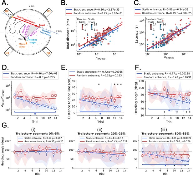
Kinetic and geometric features and correlation with active sensing.
(A) Definition of the geometric features that measure performance across trials. Food line: the straight line that connects the food hole (target) to the entrance; this line defines the optimal trajectory and minimum distance from start to target, . Distance to food line: minimum (perpendicular) distance from the mouse center to the food line (it can be regarded as the trajectory ‘error’, or deviation, from the optimal trajectory). M-T line: a line that connects the mouse center to the target. Mouse vector: a vector that points from the mouse center to its nose. Heading angle: angle between the mouse vector and the M-T line (heading angle = 0 means going straight to the target). (B) The total traveled distance correlates with the number of checked holes for every trial, sampling all mice together in both random and static entrance experiments. (C) The total trial time spent before reaching the food almost linearly correlates with the number of checked holes for every trial: regardless of how long the mouse runs, they keep checking the arena for food. This is evidence of path integration because even after learning, the mice are still uncertain, so they keep checking. In the main text and in Figure 3—figure supplement 1, we showed that these checks in later trials accumulate near (<20 cm) the target. (D, E, F) Comparison of the evolution of kinetic and geometric parameters across trials, averaging each performance feature over mice (N=8; symbols = mean; shaded region = full extent of the sample; error bars = standard deviation). (D) The traveled distance (D) becomes quasi-optimal in the static entrance case, approaching . (E) The heading angle to the food line decreases significantly only in the static case. (F) The heading angle decreases significantly only in the static case. Asterisks mark significant differences between random and static cases (q<0.05, FDR-corrected); stars mark significant differences between first and last trials of the same case (p<0.05). (G) Heading angle averaged over mice displayed as a function of trials for different segments of the trajectory: (i) 0–5%; (ii) 20–25%; and (iii) 80–85%. A segment is defined as the percentage of the latency (i.e. total trial time). For example, the 0–5% comprises only the part of the trajectory between the start and 5% of the total trial time shown in C. Only in the last parts of the trajectories the mice turn to the food (evidenced by a significant decrease of the heading angle vs. trials in the 80–85% segment), suggesting that the mice tend to keep their trajectories variable.
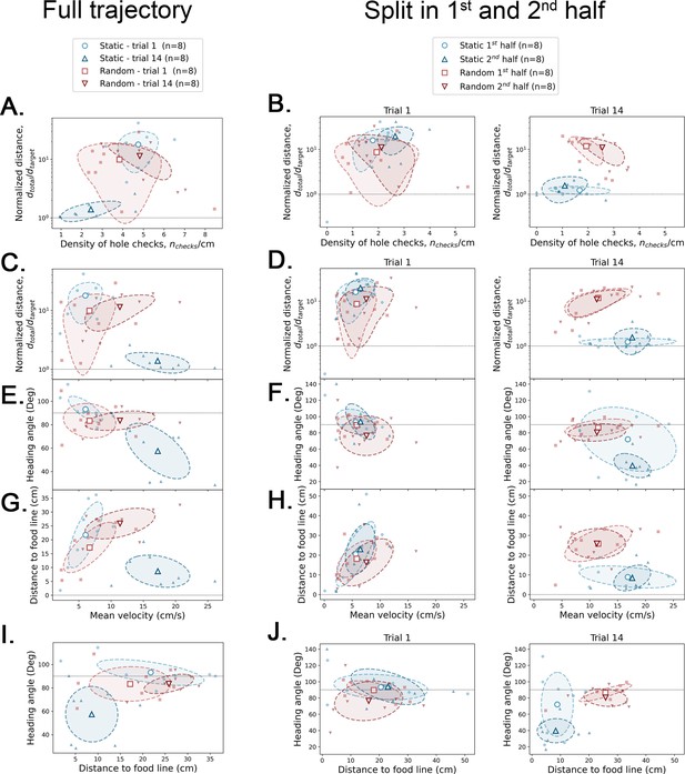
Covariance between geometric and kinetic features, and active sensing.
The definition of each of these parameters is given in Figure 4—figure supplement 3. Small filled symbols = average over trajectory for each mouse; large empty symbols = average over mice (N=8) of small symbols. Dashed ellipsis = covariance across mice. Left column: full trajectory analysis – each feature is averaged over the whole trajectory of each mouse. Center and right columns: half trajectory analysis – each feature is averaged over the first and second half of the trajectory for trial 1 (center) and trial 14 (right). The four large empty symbols give the average over the eight mice for each case. Horizontal dotted lines are there for reference values.
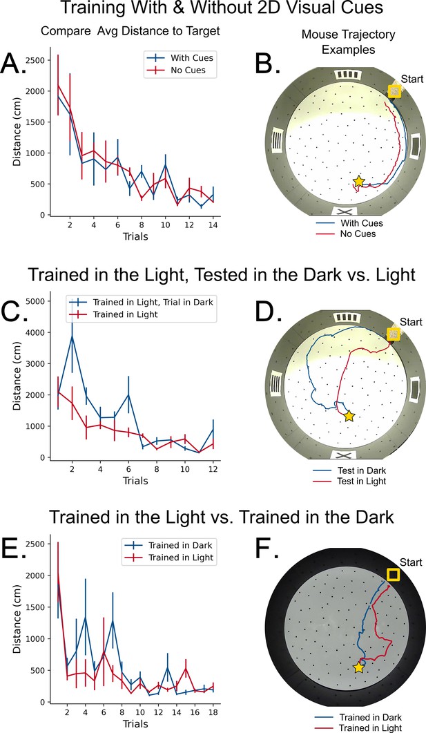
Control experiments for path-integration.
(A) Comparison in learning rate between mice with 2D cues on the wall (blue) and mice with no cues (red). N=4 mice per group, Error = SE. No significant difference in performance. (B) Example trajectories of mice trained with and without 2D visual cues. (C) Comparison in learning rate between two groups of mice trained in the light. N=4 mice per group, Error = SE. No significant difference in performance. (D) An example trajectory of a mouse trained in the light successfully navigating towards the target in darkness (blue line). A control trajectory of a mouse navigating in the light is shown (red line). (E) Comparison in learning rate between mice trained and tested in complete darkness versus mice trained in light and tested in light. The trained and tested in darkness mice had additional controls for potential odor cues (see Materials and methods). N=4 mice per group, Error = SE. No significant difference in performance. (F) Example trajectories of mice trained and tested in darkness versus trained and tested in light successfully traveling towards the target in both darkness (blue line) and light (red line), respectively.
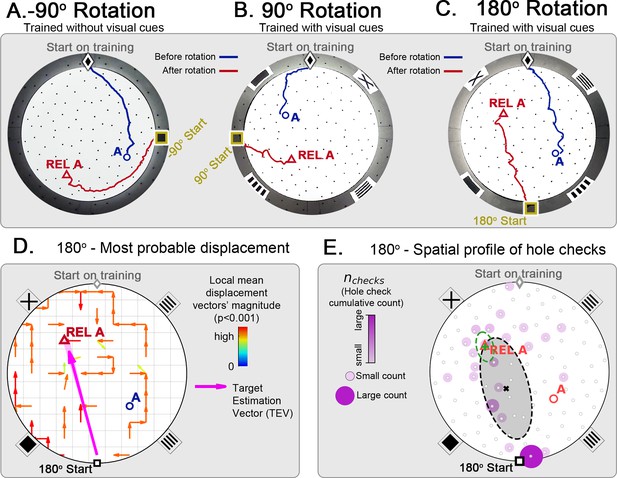
Changing start position after training in static protocol.
Mice are trained in the static entrance protocol to find food at the target labeled ‘A’ (blue circle), and a probe trial is executed with mice entering from a rotated entrance after 18 trials. (A, B, C) show the comparison between trajectories from the last learning trial (blue) versus the probe (red). The training was performed without landmarks (A) N=8, –90o rotation and with landmarks (B) N=8, 90o rotation; (C) N=8, 180o rotation. In all instances, mice ignored landmarks and went to the REL location (“REL A” label, red triangle), something that is expected under the path integration hypothesis. (D) Trajectory directionality analysis and TEV (pink arrow; shaded sector: S.D.) show that significant paths of all mice (p<0.001; N=8; see Materials and methods) point to the REL-A location in the same way that it pointed to the target without rotated entrance in Figure 4F. (E) The spatial distribution shows that hole checks accumulate along the start-REL vector, instead of the start-target vector of the case without rotation in Figure 4H. Black ellipse (x=mean): covariance of hole check distribution. Green ellipse (+=mean): covariance of the data within 20 cm of the REL-A location. This suggests that mice follow trajectories anchored to their start location (idiothetic frame of reference).
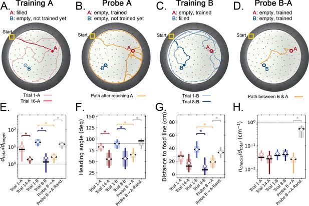
Two food location experiment.
(A-D) Trajectory exemplars of four sequential stages of the experiment (all trials done with static entrance, N=8): (A) training target A (trials 1 A and 16 A for early and late learning, respectively); (B) probe A (no food is found, triggering a random search); (C) training target B (keeping A empty; trials 1-B and 8-B for early and late learning); (D) probe B-A (where both targets are trained and empty, and the mice take a shortcut from B to A; see Figure 2—figure supplement 1 for all exemplars). Filled circles = filled target hole; empty circles = empty target. In the A and B learning stages, the trajectories evolve from random to going straight from start to the respective target. (E,F) Standard boxplot statistics of learning versus probe (diamonds are averages; asterisks: p<0.05 in a paired t-test comparison). Quantities are defined in Figure 4—figure supplement 3A. Significant differences between early and late learning were observed for the traveled distance (E), heading angle (F), and distance to the food line (G). Density of hole checks (H) remained nearly constant, as expected. In all instances, the values of all quantities in the B-A probe resembled the values of the late learning trials, whereas the randomized B-A probe (gray) had values that resembled early learning, suggesting the B-A behavior is not random. In the Probe B→A trials, the ‘food line’ is the straight line that connects B to A, along which the reference distance is measured between A and B. In the other trials, the food line is a straight line from start to the specific target, either A or B, along which is measured between start and target.
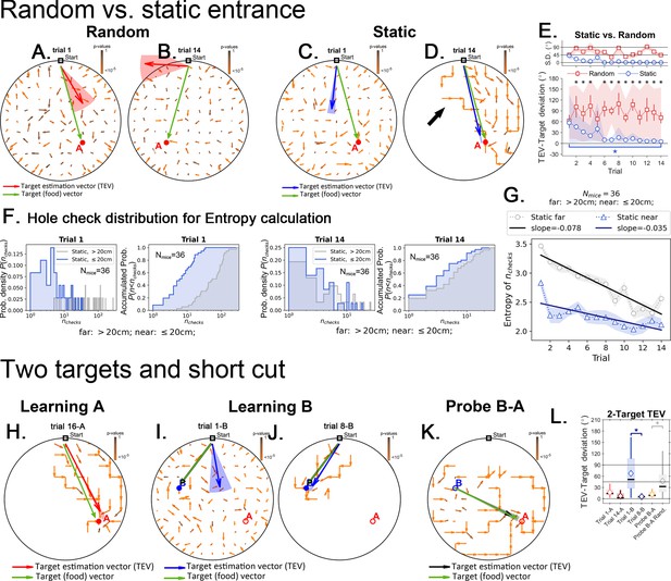
Target estimation vector (TEV) in detail for the random, static and two-target experiments.
Black arrows point to the mean displacement direction starting from any given site in the arena. Panels (A-D) and (H-K) green arrows are the target (food) vectors (point from start to target; or from B->A in the Probe B-A trial) and are to be compared with the TEVs. These panels have the same data as in Figures 4 and 7, respectively, although here all the mean displacement vectors are displayed without censoring large p values. Here, the color of the arrows corresponds to p-values (brown = 1; orange = 0). In the main text, only displacements with very small p-values are shown (see main text and Materials and methods). Panels A and B show the random entrance condition. The TEV (red) reflects the learned target position, and does not correspond with the food vector, highlighting a random search pattern. Panels C and D show the static entrance condition. The TEV (blue) becomes closely aligned with the food vector during late training (panel D). The big black arrow highlights how trajectories are still variable even after learning the TEV. The variation observed in trajectories result in a TEV pointing almost directly to the food; error is 11 cm – the size of the lattice site, corresponding roughly to the average distance between nearest holes. (E) The angle between food vector and TEV in both random and static conditions as training progresses. Angle differences decrease in the static case but not in the random case. N=8 per group, significant differences are marked with an asterisk (FDR corrected, q<0.01). The star marks significant difference between first and last trials only for the static entrance case. (F) Distribution of the number of hole checks, P(nchecks) near the target (≤20 cm) vs. far for all experiments in static entrance experiment (N=36 mice). (G) Entropy related to the distributions in panel F, H = -ΣP(nchecks)log[P(nchecks)], where the sum runs over all values of nchecks. The entropy of the number of hole checks is always lower for the near compared to far hole checks. In other words, the mice are more consistent in choosing the numbers of holes to check when near the food site (<20 cm) versus further from the food (>20 cm). The entropy decays for both far and near the target conditions consistent with learning food location over trials, but the decay is twice as steep for the far condition. The cumulative densities are shown next to the probability densities. (H) In the static condition the TEV (red) points to the learned location of the target A (analogous to Static target in panel D). (I,J) First and last training trials of target B (after completing training of target A). The TEV (in blue) starts pointing to A (trial 1B), but ends up pointing to B (trial 8B). Panel K. No food probe trial. The mean displacement generates a TEV (orange vector) that points from site B to A, highlighting the shortcut route. Panel L. Learning vs. shortcut. The difference in angle between the food vector and the TEV. The difference becomes significantly lower as training progresses, going back up as the target is switched from A to B, and then going down again as the mice learn the new target. During the probe trial, the TEV-target angle is as small as the late learning trials of either target B or target A (i.e. when the mice know their route). The TEV for the probe trial is significantly smaller than a TEV generated using a random step map (gray box, see Materials and methods for how a random step map was generated).
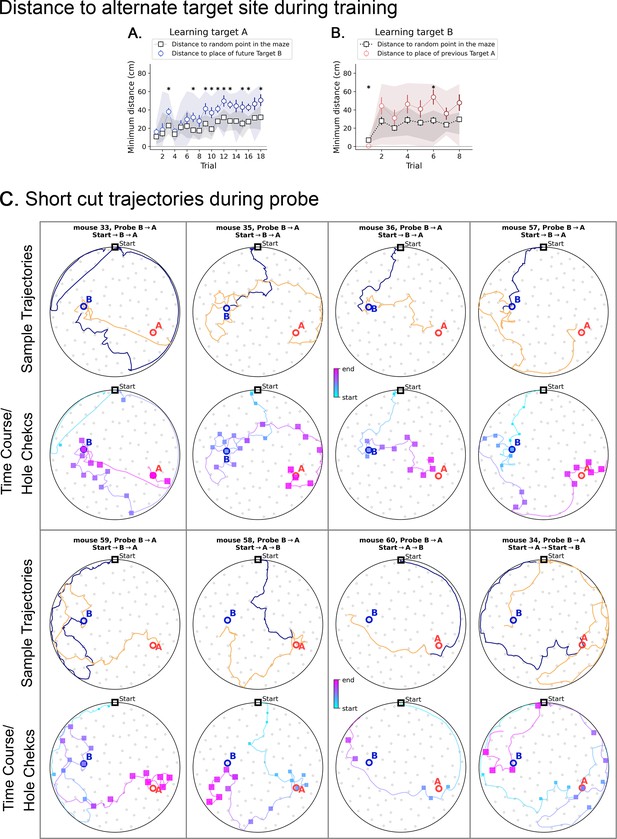
Minimum distance to alternative target in 2-target condition, and short cut trajectories.
(A and B) Black squares are the minimum distances expected by chance for each trial; they are calculated with respect to a random point, and then averaged over ten such random points. Shaded area represents the range of values, and bars represent the standard deviation. (A) During the learning of target A (no previous target has been presented), the mice keep consistently farther than expected by chance from the location where Target B will be placed (blue circles; asterisks show significant differences to chance). (B) The same pattern repeats when learning target B (target A has been already learned and is not present anymore): the mice keep consistently farther than expected by chance from the location where the previous Target A was found (red circles; asterisks show significant differences to chance). During the learning of B, some mice did visit the A location sporadically, making the shaded area larger in panel B. However, they did not rely on target A to find B. (C) Short cuts and active sensing for the Probe B→A trial. For each mouse, the plots in the top arenas contain trajectories split into two parts: before (blue) and after (orange) the visit to the first target (either A or B, whichever comes first, colored in blue). The bottom arenas of each mouse contain the time course blue is early and pink is late with hole checks in squares (blue is early and pink is late) to give a sense of when each event happened. We cut off the trajectories after visit to the last target (either A or B, whichever comes later, to ensure we observe its visit to both A and B locations). The orange trajectories are the ones that the mice took after realizing there is no food in either A or B (whichever comes earlier). We expect that mice perform the sequence Start→B→A, since B was trained last. Notice in the time course plots that mice 33, 35, 36, 57, and 59 do exactly this without ever going back to Start. Mice 34, 58, and 60 perform Start→A→B, but only mouse 34 visits the Start before heading from A to B.
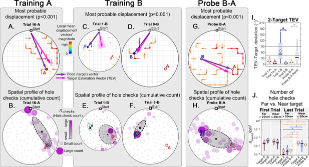
Trajectory directionality and active sensing in two food location experiment.
Arenas on the top row (mean displacement vector) correspond to the ones immediately below them (hole checking spatial distribution); the red ‘A’ and blue ‘B’ labels mark the targets (food sites), which are pointed by the target vector (purple arrow). Top row (A, C, D, G): the color and arrows indicate the most probable route taken (red = more probable; only p<0.001 displacements shown; pink arrow = inferred target position, or TEV; shaded pink sector = S.D. of TEV; see Materials and methods, and Figure 6—figure supplement 1). Bottom row (B, E, F, H): spatial distribution of hole-checks; size and color of circles = normalized frequency at which a hole was checked (larger pink circles = higher frequency); Black ellipse (x=mean): covariance of spatial distribution. Green ellipse (+=mean): covariance of spatial distribution restricted to ≤20 cm of the target. Three stages of the experiment are shown (N=8; all training done in static entrance with no landmarks): after learning the target A (A, B trial 16 A; significant routes and hole checks are observed only along the target vector, as expected); training of the target B (C, E: trial 1-B; D, F: trial 8-B); it shows the evolution of the TEV from pointing to A to pointing to B, and the hole checks distribution becomes limited to the newly learned target vector towards B; probe B-A (G, H) shows significant routes from B to A (shortcuts; N=5 out of 8 performed the route Start→B→A; see Figure 2—figure supplement 1 for all samples); hole-checks accumulated along the B-A path suggesting that mice remember both locations. (I, J) TEV-target deviation and hole-check area density, respectively. Probe B-A measures are compatible with trials where trajectories have already been learned. Standard boxplot statistics. Diamond: mean. Asterisks/star: p<0.05 (t-test).
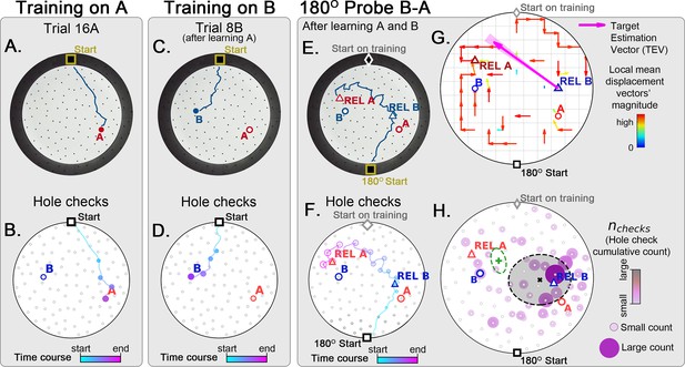
Two food location training with 180° rotated probe.
Mice (N=8) are trained to find food in the target labeled ‘A’ (red circle, panel A), and in target labeled ‘B’ (blue circle, panel B) afterwards; then a 180o rotated probe trial (no food; panel C) is realized to check whether the mice are able to generalize and take the shortcut from REL-B (blue triangle) to REL-A (red triangle), instead of the A and B targets. No landmarks are present. Panels A, C, E show exemplars of trajectories in three stages of the experiment, and B, D, F show their time course and hole-check locations marked with circles that increase with elapsed time. (G) Trajectory directionality analysis and TEV (pink arrow; shaded sector: S.D.) show that significant paths (p<0.001; N=8; see Materials and methods) point from REL-B to REL-A in the same way that it pointed from B to A without rotated entrance in Figure 7G. (H) The spatial density shows that hole checks accumulate along the REL-B to REL-A direction, instead of the B-A direction in the case without rotation in Figure 7H. Black ellipse (x=mean): covariance of hole check density. Green ellipse (+=mean): covariance of the same data restricted to ≤20 cm of the REL-A location. This suggests that mice follow shortcut trajectories anchored to their start location (idiothetic frame of reference).
Videos
The Shortcut video illustrates a two-food site experiment including hole checks; there were no landmarks.
The mouse was first trained with food at Site A (6 days, 18 trials) and, after training was complete, trained with food at Site B (3 days, 9 trials). The video was taken on a probe trial (Day 10) with no food at either Site A or Site B. The mouse is observed to proceed along a TEV to Site B with a departure from the TEV at the second hole check, followed by a third hole check as it loops back to Site B. After hole checking Site B, the mouse goes on a TEV to Site A with a departure after its third hole check. It then returns to the TEV with further hole checks. Just before reaching Site A the mouse turns and moves very slowly to a hole 16 cm from Site A; this hole check was missed by our algorithm and had to be manually added for statistics. The mouse spends ~2 s at this hole, although it had never contained food; other holes were visited for <1 s. Over the course of the experiment, the mouse visited this hole five times prior to finding the food, but did not visit it in the four trials preceding this Probe trial. Other holes within 15 cm of the target were visited at equal or greater rates. In other words, there was no special sensory input that would have made this hole interesting.
We hypothesize that this was the hole predicted by the mouse’s cognitive map to be Site A. The mouse subsequently continued to check Site A and a site near the wall. At this point the experiment was terminated. Our ‘wash and rotate the floor’ protocol to eliminate odor trails or ‘floor scratch cues’ results in the floor of the maze being washed and rotated 108 times from the first Site A learning trial to the final Probe trial when Site B and Site A were empty. The floor rotation results in the same configuration of hole positions relative to every entrance, making the environment identical at every trial for all the mice (see Materials and methods).
Note that the mouse makes its first hole check at a hole near the entrance and a final hole check near the maze wall far from an entrance. Food was never given at either site and there were no features differentiating these holes to make them ‘interesting’. These ‘near the wall’ hole checks were also seen in other mice, but we have no compelling hypothesis as to why they occur at these holes.


