A deep learning approach for automated scoring of the Rey–Osterrieth complex figure
- Methods of Plasticity Research, Department of Psychology, University of Zurich, Switzerland
- University Research Priority Program (URPP) Dynamics of Healthy Aging, Switzerland
- Neuroscience Center Zurich (ZNZ), University of Zurich and ETH Zurich, Switzerland
- Department of Computer Science, ETH Zurich, Switzerland
- Virginia Commonwealth University, United States
- Department of Health Science, Public University of Navarre, Spain
- Instituto de Investigación Sanitaria de Navarra (IdiSNA), Spain
- 'Rita Levi Montalcini' Department of Neurosciences, University of Turin, Italy
- IRCCS Istituto Auxologico Italiano, UO di Neurologia e Neuroriabilitazione, Ospedale San Giuseppe, Italy
- Huashan Hospital, China
- Smartcode, Switzerland
- University Children's Hospital Zurich, Child Development Center, Switzerland
- Rehabilitation Center, Switzerland
- University Hospital Magdeburg University Department of Neurology, Germany
- Max Planck Institute for Biological Cybernetics, Germany
- Max Planck Institute for Human Cognitive and Brain Sciences, Germany
Figures
Figure 1 with 5 supplements
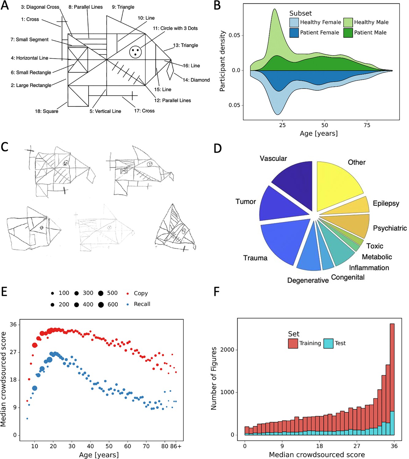
Overview of retrospective dataset.
(A) Rey–Osterrieth complex figure (ROCF) figure with 18 elements. (B) Demographics of the participants and clinical population of the retrospective dataset. (C) Examples of hand-drawn ROCF images. (D) The pie chart illustrates the proportion of the different clinical conditions of the retrospective dataset. (E) Performance in the copy and (immediate) recall condition across the lifespan in the retrospective dataset. (F) Distribution of the number of images for each total score (online raters).
Figure 1—figure supplement 1
Original scoring system according to Osterrieth.
Figure 1—figure supplement 2
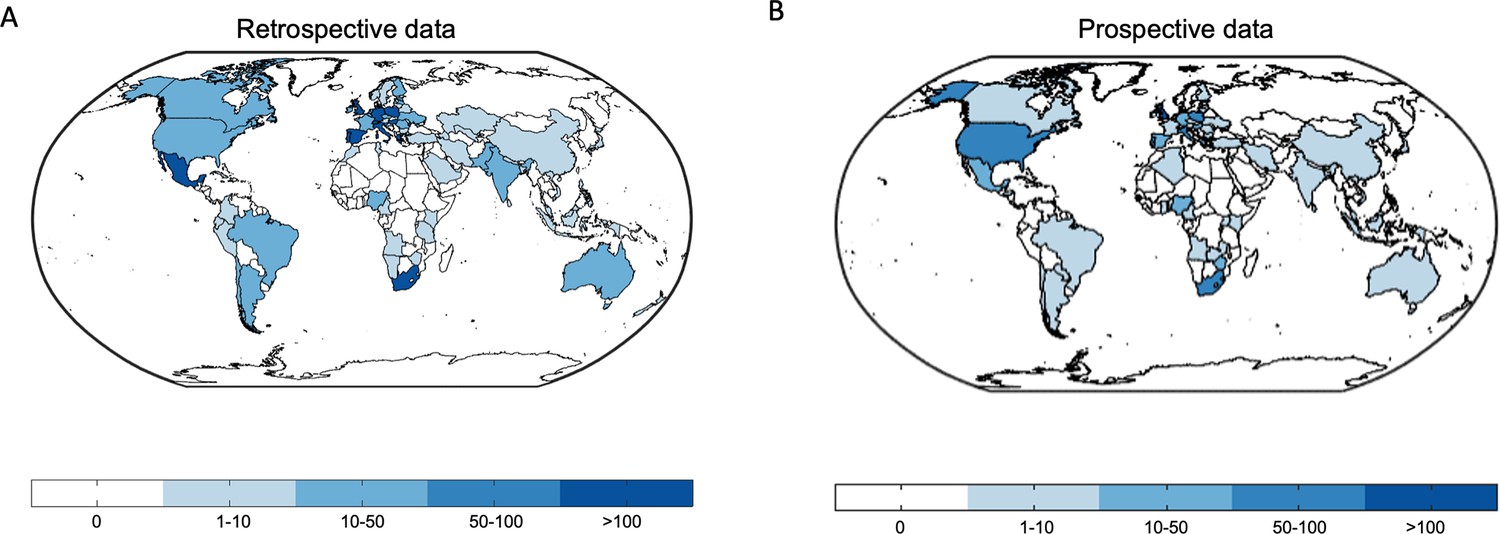
World maps depict the worldwide distribution of the origin of the data.
(A) Retrospective data. (B) Prospective data.
Figure 1—figure supplement 3

The graphical user interface of the crowdsourcing application.
Figure 1—figure supplement 4
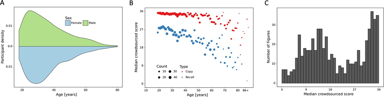
Overview of prospective dataset.
(A) Demographics of the participants of the prospectively collected data. (B) Performance in the copy and (immediate) recall condition across the lifespan in the prospectively collected data. (C) Distribution of number of images for each total score for the prospectively collected data.
Figure 1—figure supplement 5
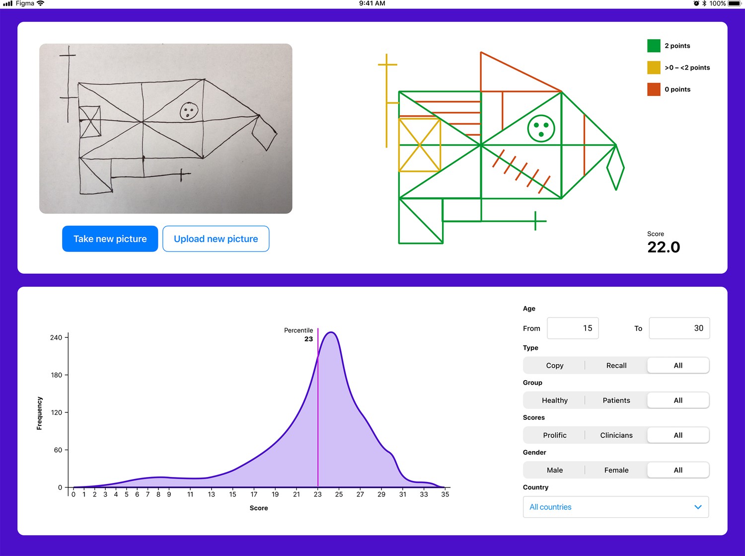
The user interface for the tablet- (and smartphone-) based application.
The application enables explainability by providing a score for each individual item. Furthermore, the total score is displayed. The user can also compare the individual with a choosable norm population.
Figure 2
Model architecture and performance evaluation.
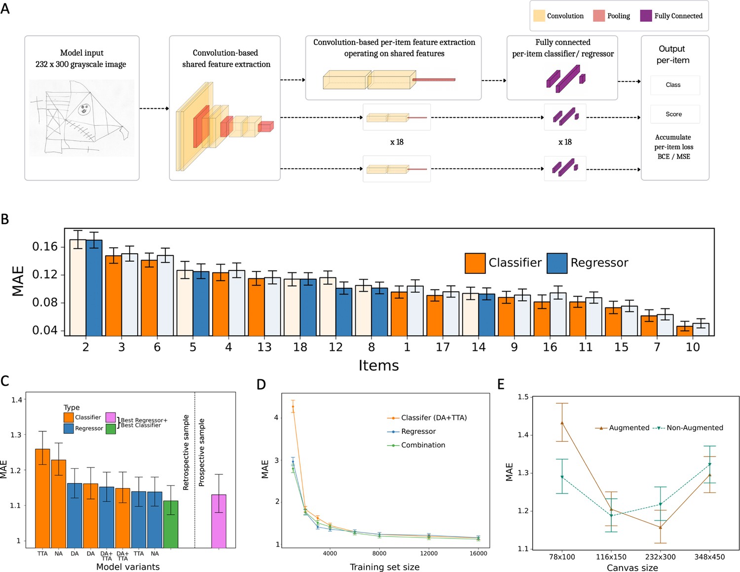
(A) Network architecture, constituted of a shared feature extractor and 18 item-specific feature extractors and output blocks. The shared feature extractor consists of three convolutional blocks, whereas item-specific feature extractors have one convolutional block with global max pooling. Convolutional blocks consist of two convolution and batch normalization pairs, followed by max pooling. Output blocks consist of two fully connected layers. ReLU activation is applied after batch normalization. After pooling, dropout is applied. (B) Item-specific mean absolute error (MAE) for the regression-based network (blue) and multilabel classification network (orange). In the final model, we determine whether to use the regressor or classifier network based on its performance in the validation dataset, indicated by an opaque color in the bar chart. In case of identical performance, the model resulting in the least variance was selected. (C) Model variants were compared and the performance of the best model in the original, retrospectively collected (green) and the independent, prospectively collected (purple) test set is displayed; Clf: multilabel classification network; Reg: regression-based network; NA: no augmentation; DA: data augmentation; TTA: test-time augmentation. (D) Convergence analysis revealed that after ~8000 images, no substantial improvements could be achieved by including more data. (E) The effect of image size on the model performance is measured in terms of MAE. The error bars in all subplots indicate the 95% confidence interval.
-
Figure 2—source data 1
The performance metrics for all model variants.
NA: non-augmented, DA: data augmentation is performed during training, TTA: test-time augmentation. The 95% confidence interval is shown in square brackets.
- https://cdn.elifesciences.org/articles/96017/elife-96017-fig2-data1-v1.xlsx
-
Figure 2—source data 2
Per-item and total performance estimates for the final model of the retrospective data.
Mean absolute error (MAE), mean squared error (MSE), and R² are estimated directly from the estimated scores.
- https://cdn.elifesciences.org/articles/96017/elife-96017-fig2-data2-v1.xlsx
-
Figure 2—source data 3
Per-item and total performance estimates for the final model with prospective data.
Mean absolute error (MAE), mean squared error (MSE), and R² are estimated directly from the estimated scores.
- https://cdn.elifesciences.org/articles/96017/elife-96017-fig2-data3-v1.xlsx
Figure 3 with 2 supplements
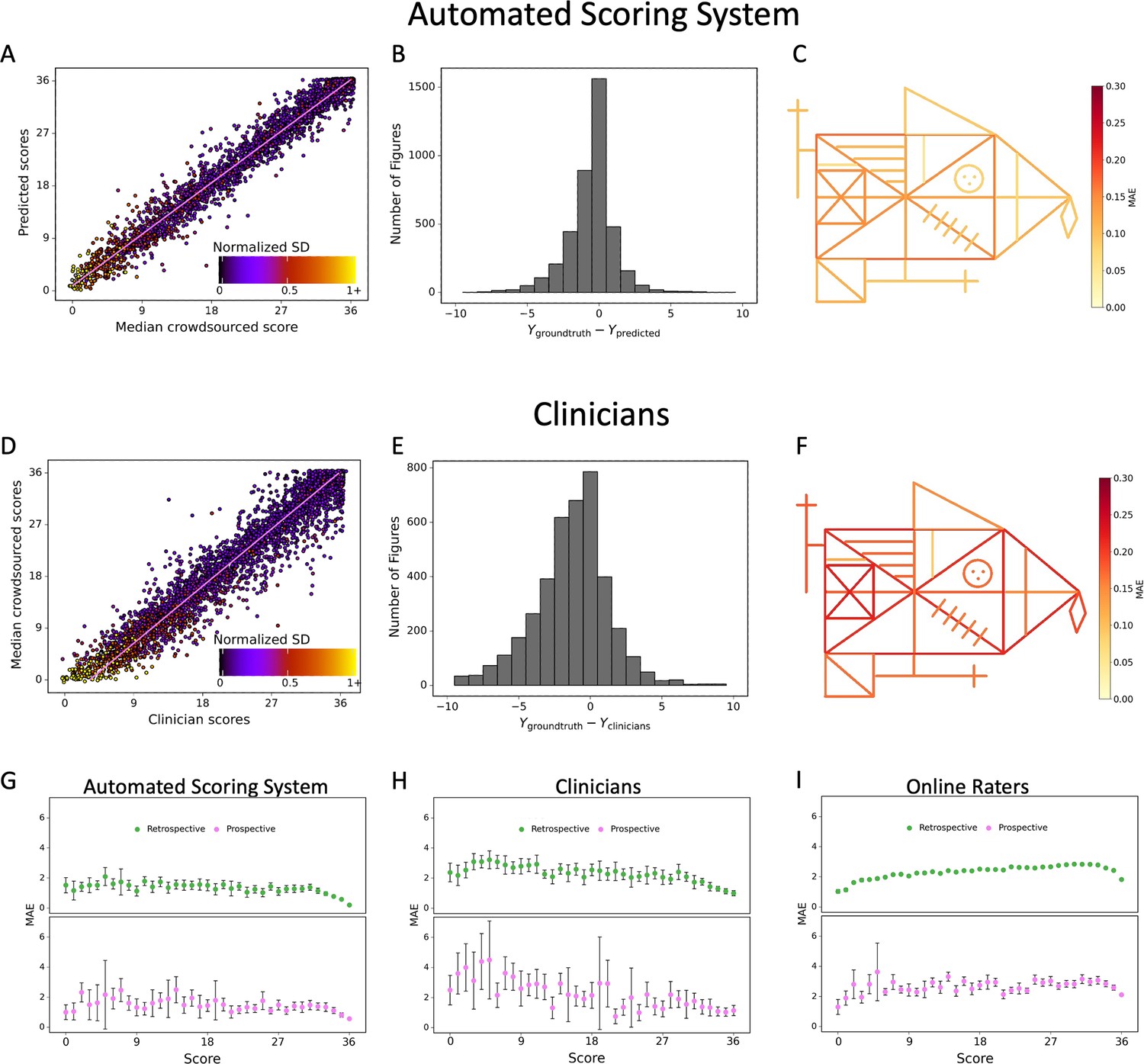
Contrasting the ratings of our model (A) and clinicians (D) against the ground truth revealed a larger deviation from the regression line for the clinicians.
A jitter is applied to better highlight the dot density. The distribution of errors for our model (B) and the clinicians ratings (E) is displayed. The mean absolute error (MAE) of our model (C) and the clinicians (F) is displayed for each individual item of the figure (see also Figure 2—source data 1). The corresponding plots for the performance on the prospectively collected data are displayed in Figure 3—figure supplement 1. The model performance for the retrospective (green) and prospective (purple) sample across the entire range of total scores for model (G), clinicians (H), and online raters (I) is presented. The error bars in all subplots indicate the 95% confidence interval.
-
Figure 3—source data 1
Performance per total score interval with retrospective data.
Thirty-seven intervals were evaluated, across the whole range of scores. We evaluated mean absolute error (MAE) and mean squared error (MSE) for the total score within each interval.
- https://cdn.elifesciences.org/articles/96017/elife-96017-fig3-data1-v1.xlsx
-
Figure 3—source data 2
Performance per total score interval with prospective data.
Thirty-seven intervals were evaluated, across the whole range of scores. We evaluated mean absolute error (MAE) and mean squared error (MSE) for the total score within each interval.
- https://cdn.elifesciences.org/articles/96017/elife-96017-fig3-data2-v1.xlsx
Figure 3—figure supplement 1
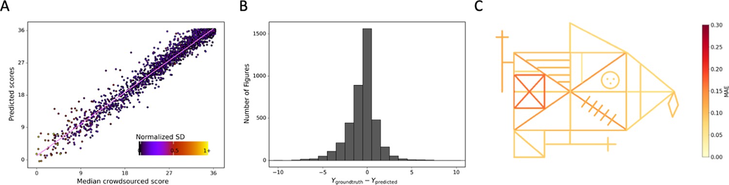
Detailed performance of the model on the prospective data.
Contrasting the ratings of our model. (A) Against the ground truth. A jitter is applied to better highlight the dot density. (B) The distribution of errors for our model on the prospective data is displayed. (C) The mean absolute error (MAE) of our model is displayed for each individual item of the figure (see also Figure 3—source data 2).
Figure 3—figure supplement 2
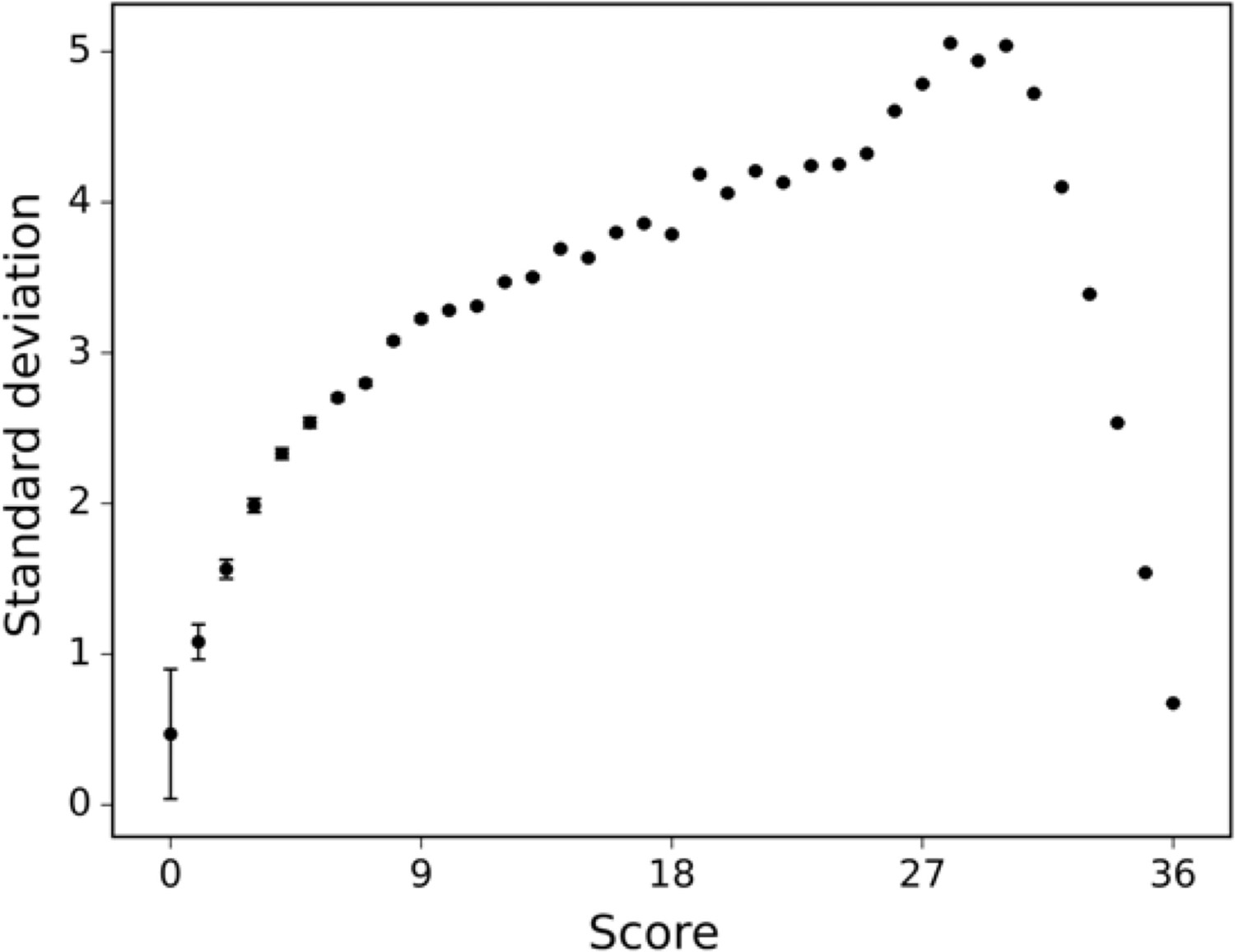
The standard deviation of the human raters is displayed across differently scored drawings.
Figure 4 with 1 supplement
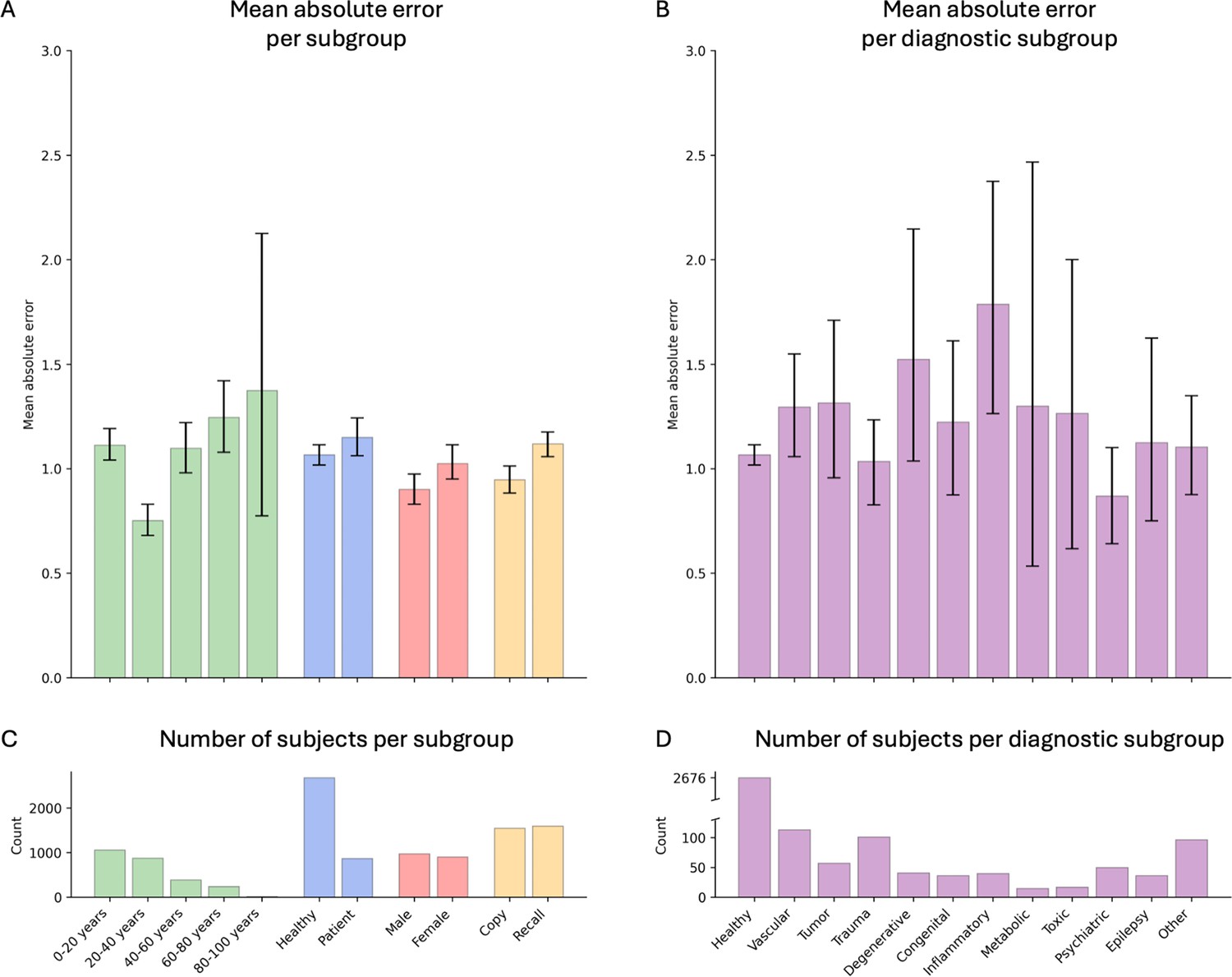
Model performance across ROCF conditions, demographics, and clinical subgroups in the retrospective dataset.
(A) Displayed are the mean absolute error and bootstrapped 95% confidence intervals of the model performance across different Rey–Osterrieth complex figure (ROCF) conditions (copy and recall), demographics (age and gender), and clinical statuses (healthy individuals and patients) for the retrospective data. (B) Model performance across different diagnostic conditions. (C, D) The number of subjects in each subgroup is depicted. The same model performance analysis for the prospective data is reported in Figure 4—figure supplement 1.
Figure 4—figure supplement 1
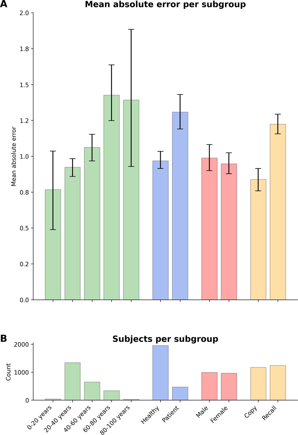
Model performance across ROCF conditions, demographics, and clinical subgroups in prospective dataset.
(A) Displayed are the mean absolute error and bootstrapped 95% confidence intervals of the model performance across different Rey–Osterrieth complex figure (ROCF) conditions (copy and recall), demographics (age and gender), and clinical statuses (healthy individuals and patients) for the prospective data. (B) The number of subjects in each subgroup is depicted. Please note, that we did not have sufficient information on the specific patient diagnoses in the prospective data to decompose the model performance for specific clinical conditions.
Figure 5 with 1 supplement
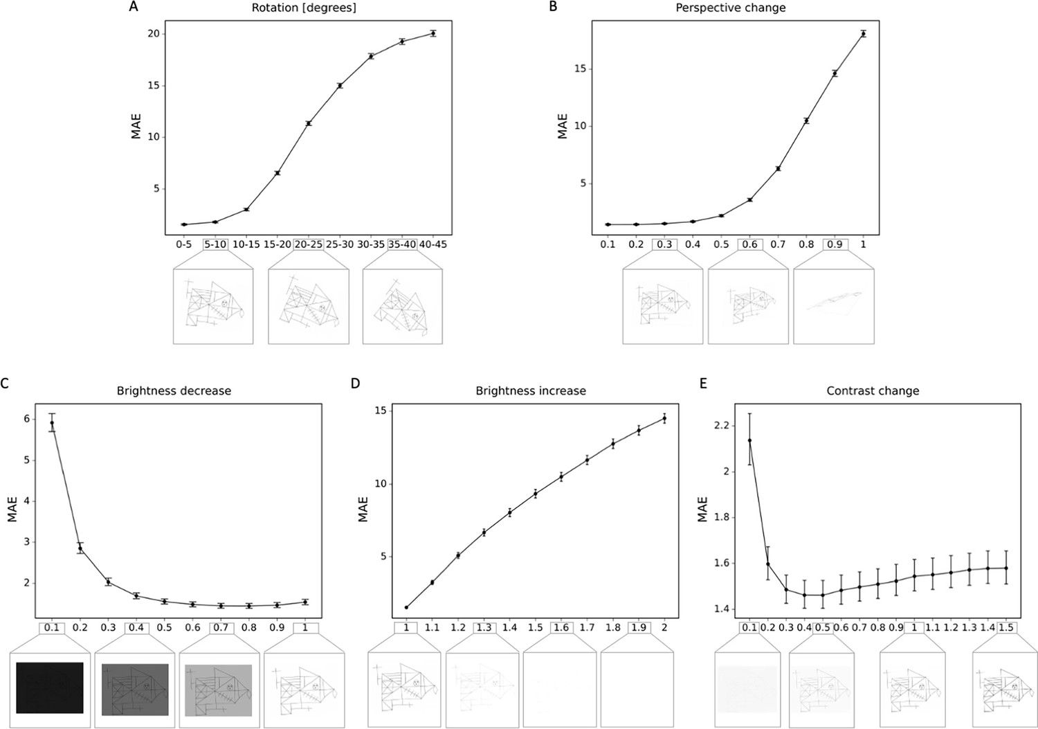
Robustness to geometric, brightness, and contrast variations.
The mean absolute error (MAE) is depicted for different degrees of transformations, including (A) rotations; (B) perspective change; (C) brightness decrease; (D) brightness increase; (E) contrast change. In addition examples of the transformed Rey–Osterrieth complex figure (ROCF) draw are provided. The error bars in all subplots indicate the 95% confidence interval.
Figure 5—figure supplement 1
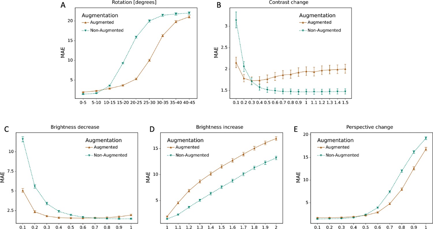
Effect of data augmentation.
The mean absolute error (MAE) for the model with data augmentation and without data augmentation is depicted for different degrees of transformations, including (A) rotations; (B) perspective change; (C) brightness decrease; (D) brightness increase; (E) contrast change.
Additional files
Download links
A two-part list of links to download the article, or parts of the article, in various formats.
Downloads (link to download the article as PDF)
Open citations (links to open the citations from this article in various online reference manager services)
Cite this article (links to download the citations from this article in formats compatible with various reference manager tools)
A deep learning approach for automated scoring of the Rey–Osterrieth complex figure
eLife 13:RP96017.
https://doi.org/10.7554/eLife.96017.3


