Convolutional networks can model the functional modulation of the MEG responses associated with feed-forward processes during visual word recognition
Figures
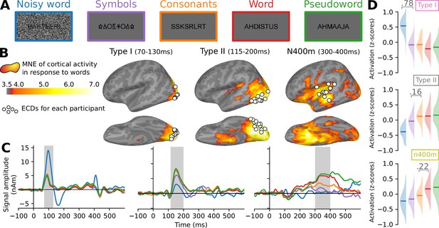
Summary of the magnetoencephalography (MEG) results obtained by Vartiainen et al., 2011.
(A) Examples of stimuli used in the magnetoencephalography (MEG) experiment. Each stimulus contained seven to eight letters or symbols. (B) Source estimate of the evoked MEG activity, using MNE-dSPM. The grand-average activity to word stimuli, averaged for three time intervals, is shown in orange hues. For each time interval, white circles indicate the location of the most representative left-hemisphere equivalent current dipoile (ECD) for each participant, as determined by Vartiainen et al., 2011. (C) Grand-average time course of signal strength for each group of ECDs in response to the different stimulus types. The traces are color-coded to indicate the stimulus type as shown in (A). Shaded regions indicate time periods over which statistical analysis was performed. (D) For each group of ECDs shown in (B), and separately for each stimulus type (different colors, see A), the distribution (and mean) of the grand-average response amplitudes to the different stimulus types, obtained by integrating the ECD signal strength over the time intervals highlighted in (C). Whenever there is a significant difference (linear mixed effects [LME] model, p < 0.05, FDR corrected) between two adjacent distributions, the corresponding difference in means is shown.
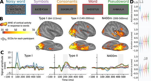
Summary of the magnetoencephalography (MEG) results on the right hemisphere.
This figure mimics Figure 1 in the paper, but contains informa tion about the right hemisphere. (A) Examples of stimuli used in the magnetoencephalography (MEG) experiment. Each stimulus contained 7–8 letters or symbols. (B) Source estimate of the evoked MEG activity, using MNE-dSPM. The grand-average activity to word stimuli, averaged for three time intervals, is shown in orange hues. For each time interval, white circles indicate the location of the most representative left-hemisphere equivalent current dipole (ECD) for each participant, as determined by Vartiainen et al., 2011. (C) Grand-average time course of signal strength for each group of ECDs in response to the different stimulus types. The traces are color-coded to indicate the stimulus type as shown in (A). Shaded regions indicate time periods over which statistical analysis was performed. (D) For each group of ECDs shown in (B), and separately for each stimulus type (different colors, see A), the distribution (and mean) of the grand-average response amplitudes to the different stimulus types, obtained by integrating the ECD signal strength over the time intervals highlighted in (C). Whenever there is a significant difference (LME model, p < 0.05, FDR corrected) between two adjacent distributions, the corresponding difference in means is shown.
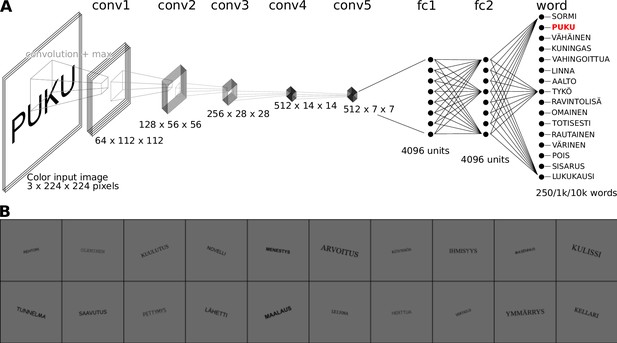
Overview of the proposed computation model of feed-forward processing during visual word recognition.
(A) The VGG-11 model architecture, consisting of five convolution layers, two fully connected layers, and one output layer. (B) Examples of the images used to train the model.
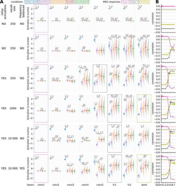
Building a model that can simulate the type I, type II, and N400m responses.
Starting from a VGG-11 model, we made adjustments to the base architecture and training diet of the model to produce variations which simulated activity better matches the response profiles of the three magnetoencephalography (MEG) evoked components. (A) For each layer, the response profile, that is the z-scored magnitude of ReLU activations in response to the same stimuli as used in the MEG experiment, is shown. Whenever there is a significant difference (t-test, p < 0.05, FDR corrected) between two adjacent distributions, the corresponding difference in means is shown. Layers for which the response pattern was qualitatively similar to that of the type I, type II, or N400m component are outlined with a box of the appropriate color. (B) Correlation between the layers of each model (horizontal axis) and the three MEG evoked components (different curves). Layers for which the response profile (A) was judged to qualitatively correspond to one of the MEG components (Figure 1D) are indicated as filled squares. Noise ceilings for the MEG components are drawn as horizontal lines.

Impact of batch normalization and noisy activations.
To accurately model the type I response profile, the model needs to filter out visual noise in its later layers.This figure explores the effect of batch normalization and having noisy unit activations on the response profiles of the model. For each layer, the response profile, that is the z-scored magnitude of ReLU activations in response to the same stimuli as used in the magnetoencephalography (MEG) experiment, is shown. Whenever there is a significant difference (t-test, p < 0.05, FDR corrected) between two adjacent distributions, the corresponding difference in means is shown. On the right side of the figure, correlation is shown between the layers of each model and the MEG evoked components. Layers which were judged to correspond to one of the MEG components are shown as filled squares. Noise ceilings for the MEG components are drawn as horizontal lines.
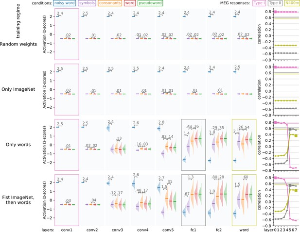
Impact of (pre-)training.
This figure shows how the response profiles of the model changes, starting from randomly initialized weights, to training with ImageNet, to training on words (10k vocabulary, frequency scaled), to pretraining on ImageNet and then training onwords. For each layer, the response profile, that is the z-scored magnitude of ReLU activations in response to the same stimuli as used in the magnetoencephalography (MEG) experiment, is shown. Whenever there is a significant difference (t-test, p < 0.05, FDR corrected) between two adjacent distributions, the corresponding difference in means is shown. On the right side of the figure, correlation is shown between the layers of each model and the MEG evoked components. Layers which were judged to correspond to one of the MEG components are shown as filled squares. Noise ceilings for the MEG components are drawn as horizontal lines.
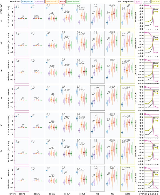
Random initializations.
The weights of the model were initialized from a model that was trained on ImageNet, so are the same every time the model is trained. However, the order of the words shown during training are random. This figure shows the variance in response profiles as the model is retrained 10 times, each time with a new random shuffling of the training words (10k vocabulary, frequency scaled). For each layer, the response profile, that is the z-scored magnitude of ReLU activations in response to the same stimuli as used in the magnetoencephalography (MEG) experiment, is shown. Whenever there is a significant difference (t-test, p < 0.05, FDR corrected) between two adjacent distributions, the corresponding difference in means is shown. On the right side of the figure, correlation is shown between the layers of each model and the MEG evoked components. Layers which were judged to correspond to one of the MEG components are shown as filled squares. Noise ceilings for the MEG components are drawn as horizontal lines.
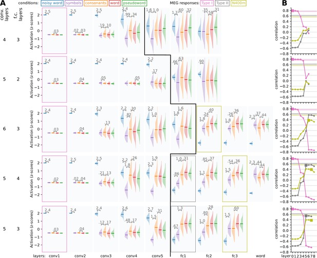
Exploring changes in model architecture.
Model variations were constructed with a different number of convolution and fully connected layers to see what architecture produces activity that is the most like the three magnetoencephalography (MEG) components. (A) For each layer, the response profile, that is the z-scored magnitude of ReLU activations in response to the same stimuli as used in the MEG experiment, is shown. Whenever there is a significant difference (t-test, p < 0.05, FDR corrected) between two adjacent distributions, the corresponding difference in means is shown. Layers for which the response pattern was qualitatively similar to that of the type I, type II, or N400m component are outlined with a box of the appropriate color. A black line separates convolution layers from fully connected layers. (B) Correlation between the layers of each model (horizontal axis) and the three MEG evoked components (different curves). Layers for which the response profile (A) was judged to qualitatively correspond to one of the MEG components (Figure 1D) are indicated as filled squares. Noise ceilings for the MEG components are drawn as horizontal lines.
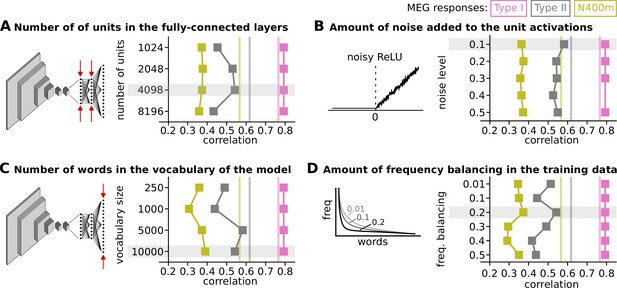
Impact of several hyperparameters on the correlation between model and brain.
This figure shows the correlation between the response profiles of the type I, type II, and N400m evoked magnetoencephalography (MEG) components and the three layers in the models whose response profiles best match each of the MEG components. Estimated noise ceilings for each of the MEG components are shown as vertical lines. Each panel shows the impact of tweaking a hyperparameter and has an illustration to indicate the property of the model affected by the hyperparameter. The settings of the hyperparameters chosen for the final modal are highlighted in gray. (A) The number of units in the two fully-connected layers, the bottleneck, is being modulated. The impact of the number of units in the two fully-connected layers, the bottleneck, is being modulated. (B) The impact of the amount of noise (σnoise) added to the activation of the units. (C) The impact of the number of words in the vocabulary of the model. (D) The impact of the amount of frequency balancing () in the training data.
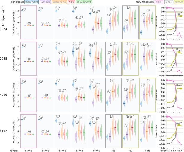
Impact of fully connected layer width on model response profiles.
Impact of fully connected layer width on model response profiles. As the vocabulary of the model (10,000) exceeds the number of units in the fully connected layers, a bottleneck is created in which a sub-lexical representation is formed. This figure shows how the response profiles of the model change as a function of the width of this bottleneck. For each layer, the response profile, that is the z-scored magnitude of ReLU activations in response to the same stimuli as used in the magnetoencephalography (MEG) experiment, is shown. Whenever there is a significant difference (t-test, p < 0.05, FDR corrected) between two adjacent distributions, the corresponding difference in means is shown. On the right side of the figure, correlation is shown between the layers of each model and the MEG evoked components. Layers which were judged to correspond to one of the MEG components are shown as filled squares. Noise ceilings for the MEG components are drawn ashorizontal lines.
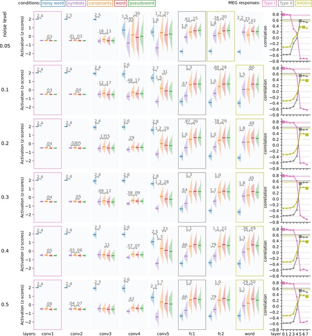
Impact of amount of noise in the unit activations on model response profiles.
To accurately model the type I response profile, the model needs to filter out visual noise in its later layers. This figure explores the effect of the amount of noise added to the activation of the units on the response profiles of the model. For each layer, the response profile, that is the z-scored magnitude of ReLU activations in response to the same stimuli as used in the magnetoencephalography (MEG) experiment, is shown. Whenever there is a significant difference (t-test, p < 0.05, FDR corrected) between two adjacent distributions, the corresponding difference in means is shown. On the right side of the figure, correlation is shown between the layers of each model and the MEG evoked components. Layers which were judged to correspond to one of the MEG components are shown as filled squares. Noise ceilings for the MEG components are drawn as horizontal lines.
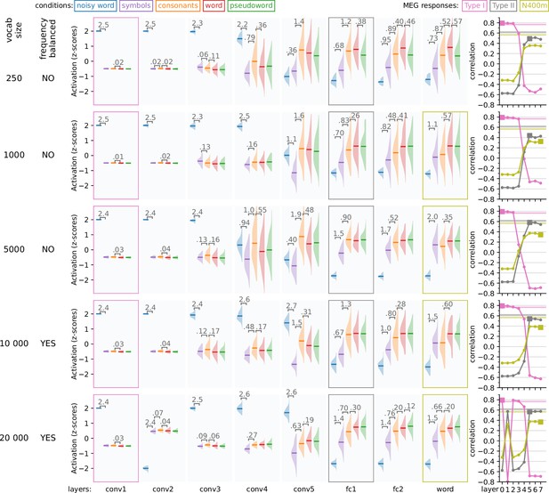
Impact of vocabulary size on model response profiles.
This figures explores the impact of vocabulary size, that is the number of word-forms in the training data and number of units in the output layer of the model. For each layer, the response profile, that is the z-scored magnitude of ReLU activations in response to the same stimuli as used in the magnetoencephalography (MEG) experiment, is shown. Whenever there is a significant difference (t-test, p < 0.05, FDR corrected) between two adjacent distributions, the corresponding difference in means is shown. On the right side of the figure, correlation is shown between the layers of each model and the MEG evoked components. Layers which were judged to correspond to one of the MEG components are shown as filled squares. Noise ceilings for the MEG components are drawn as horizontal lines.
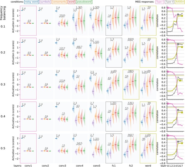
Impact of amount of frequency balancing on model response profiles.
For large vocabularies, we found it beneficial to apply frequency balancing of the training data, meaning that the number of times a word-form appears in the training data is scaled according to its frequency in a large text corpus. However, this cannot be a one-to-one scaling, since the most frequent words occur so much than other words that the training data would consist of mostly the top-10 most common words, with less common words only occurring once or not at all. Therefore, we decided to scale not by the frequency directly, but by where 0 < s < 1. This figure explores the effect of the s parameter. For each layer, the response profile, that is the z-scored magnitude of ReLU activations in response to the same stimuli as used in the magnetoencephalography (MEG) experiment, is shown. Whenever there is a significant difference (t-test, p < 0.05, FDR corrected) between two adjacent distributions, the corresponding difference in means is shown. On the right side of the figure, correlation is shown between the layers of each model and the MEG evoked components. Layers which were judged to correspond to one of the MEG components are shown as filled squares. Noise ceilings for the MEG components are drawn as horizontal lines.
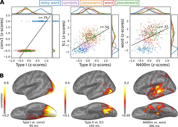
A closer look at the relationship between the final model and magnetoencephalography (MEG) responses.
(A) A closer look at the relationship between the response profiles of the MEG responses and three layers of the model that qualitatively best capture those MEG responses. Kernel density distributions are shown at the borders. (B) Correlation between the MNE-dSPM source estimate and the model. Grand-average source estimates were obtained in response to each stimulus. The correlation map was obtained by correlating the activity at each source point with that for the chosen three layers of the model. The correlation map is shown at the time of peak correlation (within the time windows indicated in Figure 1C). Only positive correlations are shown.
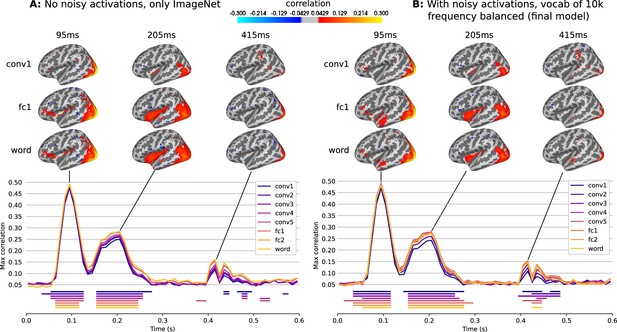
Brainscore.
A visualization of the brainscores between two models and the single-participant, single-trial evoked responses, source localized using MNE-dSPM (MNE-Python). The first model shown (A) is an illiterate model, trained only on ImagetNet, which is the model shown in the first row of Figure 3 in the main manuscript. The second model (B) is the final model, as shown in the last row of Figure 3 in the main manuscript. Brainscores were computed by training a ridge regression model on the average evoked responses of 14 participants and computing the correlation between the predicted and true responses for the 1 left-out participant (SciKit-Learn). The shrinkage parameter of the regresion model was determined using inner leave-one-out cross validation. At the top are maps of the brainscores for three layers of the model at three time points and below is the time course of maximum brainscores (across all source points) for each layer of the model. Cluster permutation tests were used to determine clusters of brainscores that were significantly different from zero (clustering t-value threshold of 4, α threshold of 0.05 for determining significant clusters). The temporal extent of the significant clusters is indicated with horizontal lines.
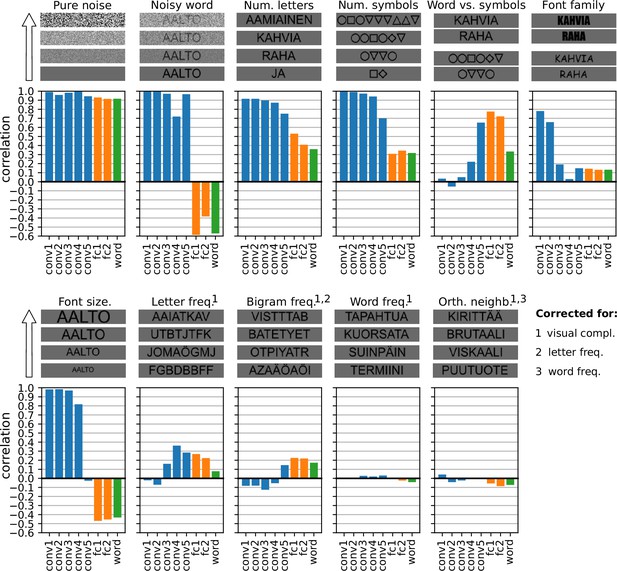
Post hoc exploration of various experimental contrasts.
For each contrast, four sample stimuli are shown to demonstrate the effect of the manipulated stimulus property and below are the correlation between the manipulation and the amount of activity in each layer of the final model. For the experimental contrasts indicated with a number, one or more confounding factors were corrected for (partial correlation). Different colors indicate convolution layers (blue), fully connected layers (orange), and the output layer (green).


