A multisite validation of brain white matter pathways of resilience to chronic back pain
Figures
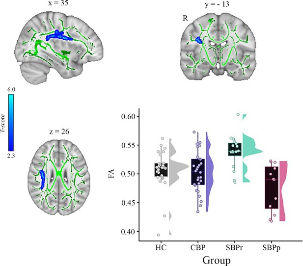
A whole brain comparison over the white matter skeleton between SBPr and SBPp patients at baseline and distribution of FA values for each group (New Haven data set).
Results of unpaired t-test (p<0.05, 10,000 permutations) showing significantly increased FA (fractional anisotropy) in SBPr (recovered) compared to SBPp (persistent) patients within the right superior longitudinal fasciculus (SLF) in the New Haven data set. Rain clouds include boxplots and the FA data distribution for each group depicted on the right side of each boxplot. Jittered circles represent single data points, the middle line represents the median, the hinges of the boxplot the first and third quartiles, and the upper and lower whiskers 1.5*IQR (the interquartile range).
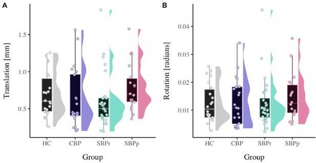
Motion parameters in the Discovery data set.
Head displacement (translation (A) and rotation (B) parameters) estimated by eddy current correction per each group in the Discovery data set (HC: healthy controls (n=28); CBP: patients with chronic back pain, (n=29); SBPr: patients with subacute back pain who recovered (n=16); and SBPp: patients with subacute back pain who developed persistent pain (n=12)). Rain clouds include boxplots and the data distribution for each group is depicted on the right side of each boxplot. Jittered circles represent single data points, the middle line represents the median, the hinges of the boxplot the first and third quartiles, and the upper and lower whiskers 1.5*IQR (the interquartile range).
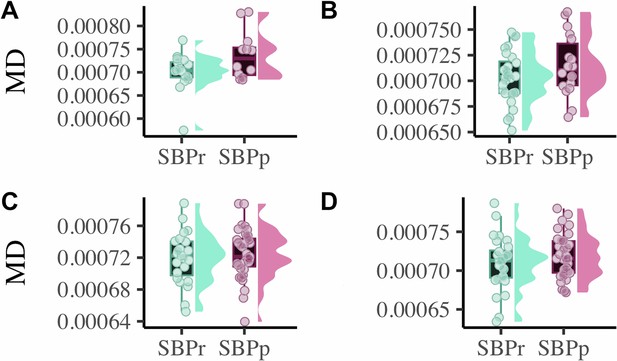
Distribution plots of mean diffusivity (MD) extracted from the RSLF mask shown in Figure 1.
The right SLF MD is significantly increased (p<0.05) in the SBPr compared to SBPp patients in the New Haven data (A). The RSLF MD is not significantly different for the Mannheim data (p=0.12) (B) nor for the Chicago data neither on visit 1 (p=0.44) (C) nor on visit 4 (p=0.38) (D). The MD values were compared between groups after accounting for age, sex, and motion parameters. The values on the plot are scaled up by 10–4 for graphical depiction. Rain clouds include boxplots and the data distribution for each group is depicted on the right side of each boxplot. Jittered circles represent single data points, the middle line represents the median, the hinges of the boxplot the first and third quartiles, and the upper and lower whiskers 1.5*IQR (the interquartile range).
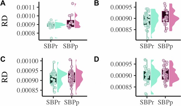
Distribution plots of radial diffusivity (RD) extracted from the RSLF mask shown in Figure 1.
The right SLF RD is significantly decreased (p<0.05) in the SBPr compared to SBPp patients in the New Haven data (A). The RSLF RD is not significantly different for the Mannheim data (p=0.24) (B). The RSLF RD is not significantly different in the Chicago data neither on visit 1 (p=0.78) (C) nor on visit 4 (p=0.70) (D). The RD values were compared between groups after accounting for age, sex, and motion parameters. The values on the plot are scaled up by 10–4 for graphical depiction. Rain clouds include boxplots and the data distribution for each group is depicted on the right side of each boxplot. Jittered circles represent single data points, the middle line represents the median, the hinges of the boxplot the first and third quartiles, and the upper and lower whiskers 1.5*IQR (the interquartile range).
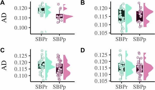
Distribution plots of axial diffusivity (AD) extracted from the RSLF mask shown in Figure 1.
The RSLF AD is not significantly different (p=0.28) in the SBPr compared to SBPp patients in the New Haven data (A). The RSLF AD (p=0.62) is not significantly different for the Mannheim data (B) nor for the Chicago data neither on visit 1 (p=0.15) (C) nor on visit 4 (p=0.36) (D). The AD values were compared between groups after accounting for age, sex, and motion parameters. The values on the plot are scaled up by 10–3 for graphical depiction. Rain clouds include boxplots and the data distribution for each group is depicted on the right side of each boxplot. Jittered circles represent single data points, the middle line represents the median, the hinges of the boxplot the first and third quartiles, and the upper and lower whiskers 1.5*IQR (the interquartile range).
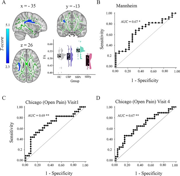
TBSS analysis and RSLF FA validation after applying neuroCombat after pooling subjects from the three sites into one analysis.
(A) A whole brain comparison over the white matter skeleton between SBPr and SBPp patients at baseline and distribution of FA values for each group (New Haven data set). Results of unpaired t-test (p<0.05, 10,000 permutations) showing significantly increased FA (fractional anisotropy) in SBPr (recovered) compared to SBPp (persistent) patients within the right superior longitudinal fasciculus (SLF) in the New Haven data set. (B–D) ROC shows the AUC when using the mask in A to classify the SBPr and SBPp patients at each of the respective sites. *, p<0.05; **, p<0.01.
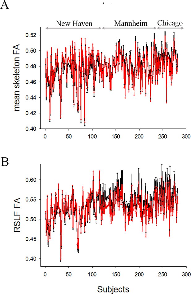
Plot of FA values before (black) and after (red) applying harmonization using neuroCombat calculated as mean skeletal FA.
(A) and right SLF FA (B). Each subject’s (x-axis) FA value (y-axis) is plotted for the 3 data sets Chicago, New Haven, and Manheim from left to right. FA values significantly changed when we compared the mean skeletal FA or right SLF FA before to after neuroCombat (paired t-test, p<10–7).
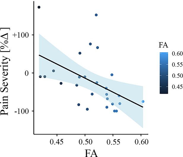
Association between white matter FA values and pain severity (New Haven data set).
Higher fractional anisotropy (FA) values in the right superior longitudinal fasciculus (SLF) are associated with greater pain reduction (from baseline to follow-up) in the New Haven data set.
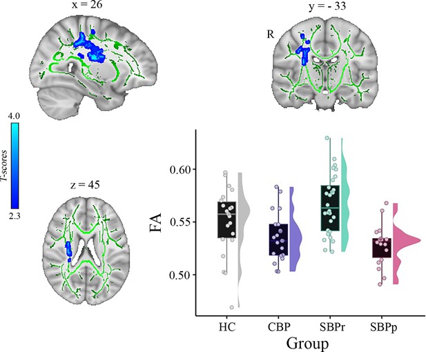
A whole brain comparison over the white matter skeleton between SBPr and SBPp patients at baseline and distribution of FA values for each group (Mannheim data set).
Results of unpaired t-test (p<0.05, 10,000 permutations) showing significantly increased FA (fractional anisotropy) in SBPr (recovered) compared to SBPp (persistent) patients at six-months follow-up within the right superior longitudinal fasciculus (SLF) in the Mannheim data set. Rain clouds include boxplots and the FA data distribution for each group depicted on the right side of each boxplot. Jittered circles represent single data points, the middle line represents the median, the hinges of the boxplot the first and third quartiles, and the upper and lower whiskers 1.5*IQR (the interquartile range).
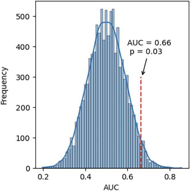
Distribution of the values of the area under the curve (AUC) when shuffling the label of the groups (recovered, persistent) using the FA values from the right SLF before neuroCombat harmonization for the Mannheim data.
The labels were shuffled 10,000 times; the p-values represent the probability of obtaining an AUC larger than the one obtained from the non-shuffled labels.
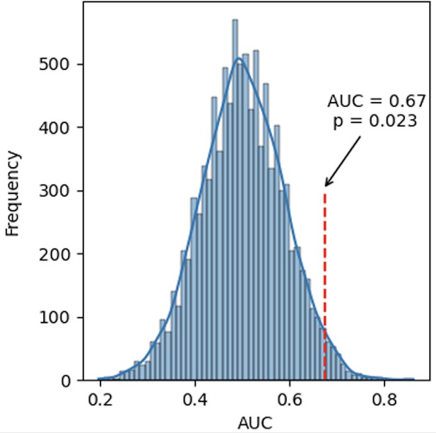
Distribution of the values of the AUC when shuffling the label of the groups (recovered, persistent) using the FA values from the right SLF after neuroCombat harmonization for the Mannheim data.
The labels were shuffled 10,000 times; the p-values represent the probability of obtaining an AUC larger than the one obtained from the non-shuffled labels.
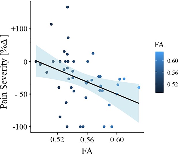
Association between white matter FA values and pain severity (Mannheim data set).
Higher fractional anisotropy (FA) values in the right superior longitudinal fasciculus (SLF) are associated with greater pain reduction (from baseline to follow-up) in the Mannheim data set.
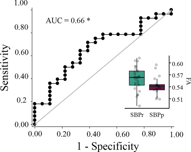
Validation of the accuracy of FA in the right SLF in classifying Mannheim patients.
The right superior longitudinal fasciculus (SLF) cluster from the discovery set accurately classifies patients who recovered (SBPr) and those whose pain persisted (SBPp) in the Mannheim data set at a 6-month follow-up. Classification accuracy is based on the ROC curve. Circles on the boxplots represent single data points, the middle line represents the median, the hinges of the boxplot the first and third quartiles, and the upper and lower whiskers 1.5*IQR (the interquartile range). AUC: area under the curve; * p<0.05.
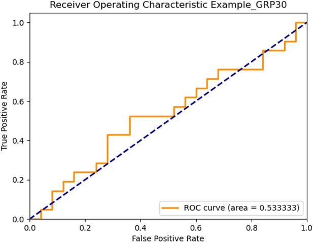
The receiver operating characteristic curve shows the area under the curve (AUC = 0.53) when using the mask from the New Haven data to classify the SBPr and SBPp patients from Mannheim using the 30% recovery criterion.
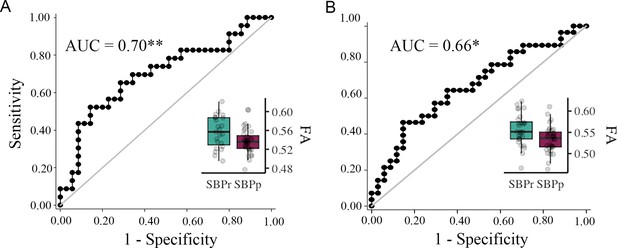
Validation of the accuracy of FA in the right SLF in classifying Chicago patients.
The right SLF (superior longitudinal fasciculus) cluster from the discovery set accurately classifies patients who recovered (SBPr) and those whose pain persisted (SBPp) in the Chicago (OpenPain) data set at visit 1 (baseline) (A) and visit 2 (one-year follow-up) (B). Classification accuracy is based on the ROC curve. Circles on the boxplots represent single data points, the middle line represents the median, the hinges of the boxplot the first and third quartiles, and the upper and lower whiskers 1.5*IQR (the interquartile range). AUC: area under the curve; * p<0.05.
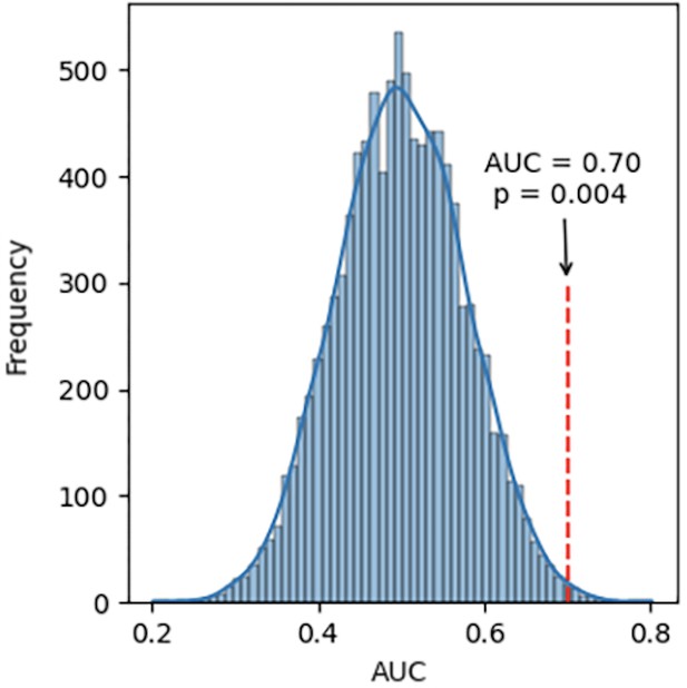
Distribution of the values of the area under the curve (AUC) when shuffling the label of the groups (recovered, persistent) using the FA values from the right SLF before neuroCombat harmonization for the Chicago data set at visit 1.
The labels were shuffled 10,000 times; the p-values represent the probability of obtaining an AUC larger than the one obtained from the non-shuffled labels.
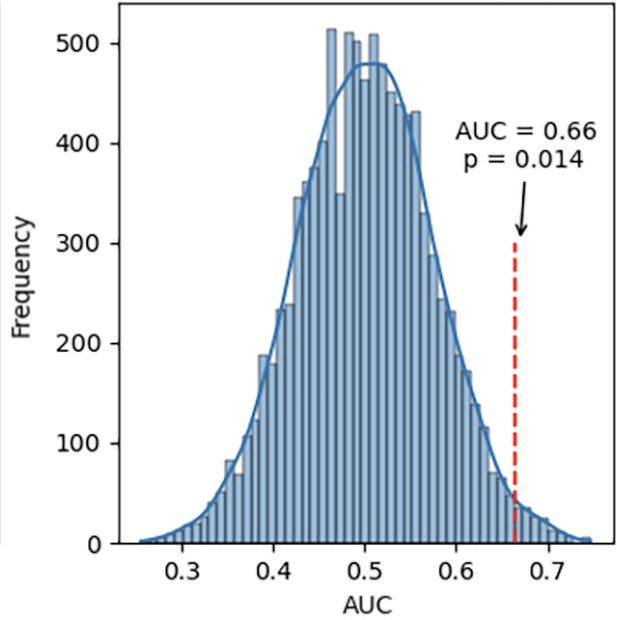
Distribution of the values of the area under the curve (AUC) when shuffling the label of the groups (recovered, persistent) using the FA values from the right SLF before neuroCombat harmonization for the Chicago data set at visit 2.
The labels were shuffled 10,000 times; the p-values represent the probability of obtaining an AUC larger than the one obtained from the non-shuffled labels.
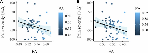
Correlation between FA values and pain severity with higher FA values (greater structural integrity) associated with the greater reduction in pain (percentage change) at baseline (n=58) (A) and follow-up (n=60) (B) in the Chicago data set.
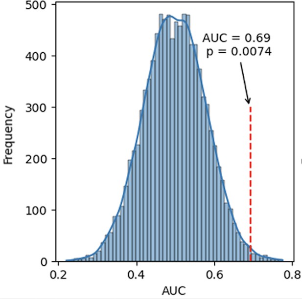
Distribution of the values of the area under the curve (AUC) when shuffling the label of the groups (recovered, persistent) using the FA values from the right SLF after neuroCombat harmonization for the Chicago data set at visit 1.
The labels were shuffled 10,000 times; the p-values represent the probability of obtaining an AUC larger than the one obtained from the non-shuffled labels.
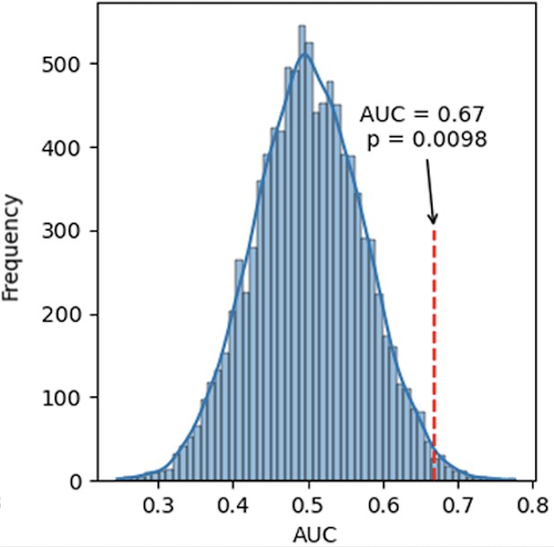
Distribution of the values of the area under the curve (AUC) when shuffling the label of the groups (recovered, persistent) using the FA values from the right SLF after neuroCombat harmonization for the Chicago data set at visit 2.
The labels were shuffled 10,000 times; the p-values represent the probability of obtaining an AUC larger than the one obtained from the non-shuffled labels.
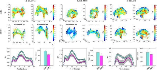
Illustration of the right SLF white matter bundles and their FA content in SBPp and SBPr patients of the New Haven data set.
(A) Three-dimensional illustration of SLF tracts connecting the inferior parietal lobe with frontal operculum (left), inferior parietal lobe and middle frontal gyrus (middle), and superior parietal lobe and primary motor cortex (right). Upper two rows show SLF tracts connecting the two regions in 3D with FA values along those tracts shown in blue-to-red. The first row shows two representative SBPr patients and the second row shows two representative SBPp patients. (B) Plot of average FA ± SEM along the tracts depicted in A for 15 SBPr and 12 SBPp patients. The histogram plot shows the average number of tracts for these same patient groups. IPL, inferior parietal lobe; PFO, prefrontal operculum; MFG, middle frontal gyrus; SPL, superior parietal lobe; M1, primary motor cortex.
-
Figure 7—source data 1
The complete list of the cortical and subcortical regions based on the Desikan-Killiany atlas (DKA) used to define the regions of interest (ROI) corresponding to the nodes in the structural connectivity analysis.
- https://cdn.elifesciences.org/articles/96312/elife-96312-fig7-data1-v1.xlsx
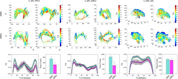
Illustration of the left SLF white matter bundles and their FA content in SBPp and SBPr patients of the New Haven data set.
(A) Three-dimensional illustration of the left (L) SLF tracts connecting the inferior parietal lobe with prefrontal operculum (left), inferior parietal lobe with middle frontal gyrus (middle), and superior parietal lobe and primary motor cortex (right). Upper two rows show SLF tracts connecting the two regions in 3-D with FA values along those tracts shown in blue-to-red. The first row shows two representative SBPr patients and the second row shows two representative SBPp patients. (B) Plot of average FA ± SEM along the tracts depicted in (A) for 15 SBPr and 12 SBPp patients. The histogram plot shows the average number of tracts for these same patient groups. IPL, inferior parietal lobe; PFO, prefrontal operculum; MFG, middle frontal gyrus; SPL, superior parietal lobe; M1, primary motor cortex.
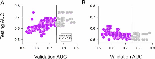
Scatterplot of the testing AUC vs. the model validation AUC for all the machine learning models applied to the structural connectivity data.
A combination of 40% of the New Haven data and 100% of the Open Pain data was used for model training and validation Testing was performed on 60% of the New Haven data.(A), and the Mannheim data (B) Each point is the result of averaging the performance of the models (i.e. AUC) across 50 iterations as the combination of the data in model training stage was bootstrapped 50 times. The green circles were the final models considered in the result sections with an initial validation AUC ≥0.75.

Schematic representation of the sequential steps performed in structural connectivity.
From left to right: data preparation, correction for confounders, and machine learning model building and testing. The dashed rectangle indicates that the combination of the data during model training was bootstrapped 50 times and validation and testing were repeated accordingly.
Tables
| Reagent type (species) or resource | Designation | Source or reference | Identifiers | Additional information |
|---|---|---|---|---|
| Software, algorithm | FSL 6.0.0 | Oxford Centre for Functional MRI of the Brain | RRID:SCR_002823 | |
| Software, algorithm | R 4.3.2 | R Foundation for Statistical Computing | RRID:SCR_001905 | |
| Software, algorithm | Python 3.11 | Python Software Foundation | RRID:SCR_008394 | |
| Software, algorithm | Original analysis code | This paper | https://www.openpain.org/ under WMPainResiliencePathway dataset | See Materials and methods, section ‘Estimation of structural connectivity’ |
New Haven sample characteristics.
| HC (N=28) | CLBP (N=28) | SBPr (N=16) | SBPp (N=12) | t(df)*, p-value | Missing | |
|---|---|---|---|---|---|---|
| Age (years) | 30.1 (10.1) | 30.7 (11.9) | 30.8 (8.8) | 38.0 (12.5) | +1.80 (26), 0.08 | 0/0/0/0 |
| Gender (m/f) | 16/12 | 12/16 | 11/5 | 7/5 | +0.32 (1), 0.57† | 0/0/0/0 |
| BMI (Kg/m2) | 24.1 (3.6) | 24.2 (3.7) | 25.5 (5.2) | 26.2 (4.5) | +0.35 (26), 0.73 | 0/0/0/0 |
| Delta pain severity: absolute | NA | NA | - 25.4 (15.4) | 8.0 (17.2) | +5.0 (26),<10–4‡ | NA/NA/0/0 |
| Delta pain severity: percentage | NA | NA | - 66.3 (26.9) | 39.1 (68.1) | +5.7 (26),<10–5‡ | NA/NA/0/0 |
| Pain Duration | NA | 5.3 (4.7) | 8.6 (3.6) | 10.9 (3.1) | +1.87 (26), 0.08 | 0/0/0/0 |
| Pain Intensity | NA | 4.5 (2.0) | 36.7 (18.8) | 33.7 (15.9) | - 0.45 (26), 0.66 | NA/0/0/0 |
| BDI | 2.6 (3.3) | 6.4 (6.0) | 7.4 (4.8) | 3.1 (3.8) | - 2.65 (26), 0.02‡ | 0/0/0/0 |
| BAI | 3.4 (5.7) | 7.6 (8.2) | 6.4 (6.8) | 4.8 (2.8) | - 0.75 (26), 0.46 | 0/0/0/0 |
| MPQ | NA | 10.6 (4.6) | 9.2 (5.2) | 9.1 (4.2) | - 0.08 (26), 0.93 | NA/0/0/0 |
| PCS | NA | 15.2 (9.8) | 12.8 (11.4) | 11.3 (8.1) | - 0.40 (26),0.69 | NA/0/1/0 |
-
Abbreviations: BMI, body mass index; BDI, Beck’s Depression Index; BAI, Beck’s Anxiety Index; MPQ, McGill Pain Questionnaire; PCS, Pain Catastrophizing Scale. Values show the group mean and standard deviation in parenthesis.
-
*
t-score (degrees of freedom).
-
†
Chi-square test.
-
‡
p < 0.05.
Mannheim sample characteristics.
| HC (N=22) | CBP (N=21) | SBPr (N=28) | SBPp (N=18) | t(df)*, p-value | Missing | |
|---|---|---|---|---|---|---|
| Age in years | 36.9 (14.4) | 40.0 (16.0) | 32.8 (12.0) | 32.1 (11.2) | +0.19 (38.2), 0.85 | 0/0/0/0 |
| Gender (m/f) | 12/10 | 11/10 | 8/20 | 6/12 | +0.0002(1),0.99* | 0/0/0/0 |
| Number of days with pain during last year | NA | 247 (84.0) | 74.8 (43.2) | 72.4 (34.9) | +0.2 (41.5,2), 0.84 | NA/1/0/0 |
| Delta pain severity (FU-BL): absolute | NA | NA | –1.90 (1.18) | 0.19 (0.71) | –7.47 (43.8),<10–9† | NA/NA/0/0 |
| Delta pain severity (FU-BL): percentage | NA | NA | –50.9 (27.3) | 8.73 (26.0) | –7.45 (37.7),<10–9† | NA/NA/0/0 |
| Pain severity (MPI) | NA | 4.92 (1.38) | 3.80 (1.43) | 3.78 (1.54) | +0.06 (34.5), 0.95 | NA/1/0/0 |
| Interference (MPI) | NA | 2.43 (1.23) | 1.48 (1.01) | 1.49 (1.00) | –0.03 (32), 0.97 | 3/0/2/2 |
| Negative mood (MPI) | NA | 2.83 (1.07) | 2.40 (1.08) | 2.71 (1.15) | –0.87 (30.5), 0.39 | 3/0/2/2 |
| Life control (MPI) | NA | 3.97 (0.971) | 4.05 (1.24) | 3.54 (1.23) | +1.3 (32), 0.2 | 3/0/2/2 |
| Support (MPI) | NA | 2.60 (1.85) | 1.85 (1.28) | 1.56 (1.41) | +0.66 (29.4), 0.52 | 3/0/2/2 |
| ÖMPQ | NA | 78.1 (19.5) | 63.6 (21.1) | 69.7 (16.1) | –1.06 (37.9), 0.3 | 12/1/2/2 |
| CPGa | NA | 1.00 [0, 6.00] | 0 [0, 4.00] | 0 [0, 6.00] | –0.65 (25.9), 0.52 | 9/0/0/2 |
| Active coping (PRSS) | NA | 3.30 (0.74) | 2.94 (0.96) | 3.14 (0.66) | –0.76 (36.6), 0.45 | NA/6/4/3 |
| Catastrophizing (PRSS) | NA | 1.35 (0.87) | 1.09 (0.73) | 1.10 (0.76) | –0.02 (28.9), 0.98 | NA/6/4/3 |
| Anxiety (HADS) | 4.37 (2.39) | 8.24 (4.47) | 7.27 (4.63) | 7.47 (3.60) | –0.15 (35.3), 0.88 | 3/0/2/3 |
| Depression (HADS) | 6.21 (6.12) | 6.00 (4.40) | 4.42 (4.23) | 4.60 (2.85) | –0.15 (37.9), 0.87 | 3/0/2/3 |
| Perceived stress (PSS) | 4.74 (5.00) | 11.0 (5.23) | 12.0 (5.25) | 11.4 (5.07) | +0.34 (32.7), 0.73 | 3/0/2/2 |
-
Chi-square test.
-
*
t-score (degrees of freedom).
-
†
p < 0.05.
Chicago (Open Pain) sample characteristics.
| SBPr (N=23) | SBPp (N=35) | t(df)*, p-value | SBPr (N=28) | SBPp (N=34) | t(df)*, p-value | Missing | |
|---|---|---|---|---|---|---|---|
| Age (years) | 41.7 (12.0) | 43.6 (9.3) | +0.7 (56), 0.48 | 43.7 (11.5) | 45.3 (9.6) | +0.61 (60), 0.54 | 0/0/0/0 |
| Gender (m/f) | 12/9 | 16/19 | 1.6 (1),0.2† | 15/13 | 17/17 | 0.08 (1), 0.78† | 0/0/0/0 |
| Delta pain severity: absolute | - 40.6 (20.8) | –3.4 (15.6) | +7.8 (56),<10–6 ‡ | - 43.1 (20.6) | - 3.2 (15.6) | +8.7 (60),<10–6‡ | 0/0/0/0 |
| Delta pain severity: percentage | - 68.9 (26.2) | –1.6 (31.9) | +8.4 (56),<10–6 ‡ | - 69.7 (25.9) | 0.3 (31.6) | +9.3 (60),<10–6‡ | 0/0/0/0 |
| Pain Duration (weeks) | 9.9 (4.1) | 8.4 (4.3) | - 1.3 (55), 0.18 | 67.8 (5.6) | 65.2 (5.7) | - 1.8 (60), 0.07 | 0/1/0/0 |
| Pain Intensity | 58.0 (15.2) | 67.7 (17.2) | +2.3 (56),0.03‡ | 18.0 (16.8) | 65.7 (15.8) | +11.5 (60),<10–6‡ | 0/0/0/0 |
| BDI | 5.7 (5.2) | 7.3 (4.6) | +1.0 (39), 0.31 | 6.3 (6.6) | 16.0 (9.5) | +1.4 (42), 0.16 | 7/10/10/8 |
| MPQ | 10.9 (4.5) | 18.2 (17.9) | +1.9 (54), 0.06 | 13.4 (26.3) | 16.0 (9.5) | +4.3 (56), <10–4 ‡ | 0/2/3/1 |
-
*
t-score (degrees of freedom).
-
†
Chi-square test.
-
‡
p < 0.05.
Summary of the type of data combinations expressed in % of subjects from each site used to build and test the brain connectivity-based machine learning models to classify recovered and persistent SBP patients.
| Training & Validation* | Testing‡ | ||||
|---|---|---|---|---|---|
| New Haven | Chicago | New Haven | Chicago | Mannheim | |
| 100% | 0% | 0% | 100% | 100% | |
| 100% | 40% | 0% | 40% | 100% | |
| 0% | 100% | 100% | 0% | 100% | |
| 40% | 100% | 60% | 0% | 100% | |
-
*
The combination of data sets was bootstrapped 50 times and the training and testing was repeated accordingly.
Additional files
-
MDAR checklist
- https://cdn.elifesciences.org/articles/96312/elife-96312-mdarchecklist1-v1.pdf
-
Supplementary file 1
Comorbid mental disorders assessment and characteristics – Mannheim data set.
A trained psychologist interviewed all participants to assess comorbid mental disorders using the German version of the Structured Clinical Interviews (SCID I) for the Diagnostic and Statistical Manual of Mental Disorders (DSM IV)(Wittchen, 1997). List of all reported diagnoses across groups is provided in Supplementary file 1—Table 1.
- https://cdn.elifesciences.org/articles/96312/elife-96312-supp1-v1.docx


