Postural adaptations may contribute to the unique locomotor energetics seen in hopping kangaroos
- School of Science, Technology, and Engineering, University of the Sunshine Coast, Australia
- School of Biomedical Sciences, University of Queensland, Australia
- Structure and Motion Lab, Department of Comparative Biomedical Sciences, The Royal Veterinary College, United Kingdom
- School of Exercise and Nutrition Science, Queensland University of Technology, Australia
- Department of Integrative Anatomical Sciences, Keck School of Medicine University of Southern California, United States
- Biomechanics Laboratory, Department of Kinesiology, The Pennsylvania State University, United States
Figures
Figure 1 with 3 supplements
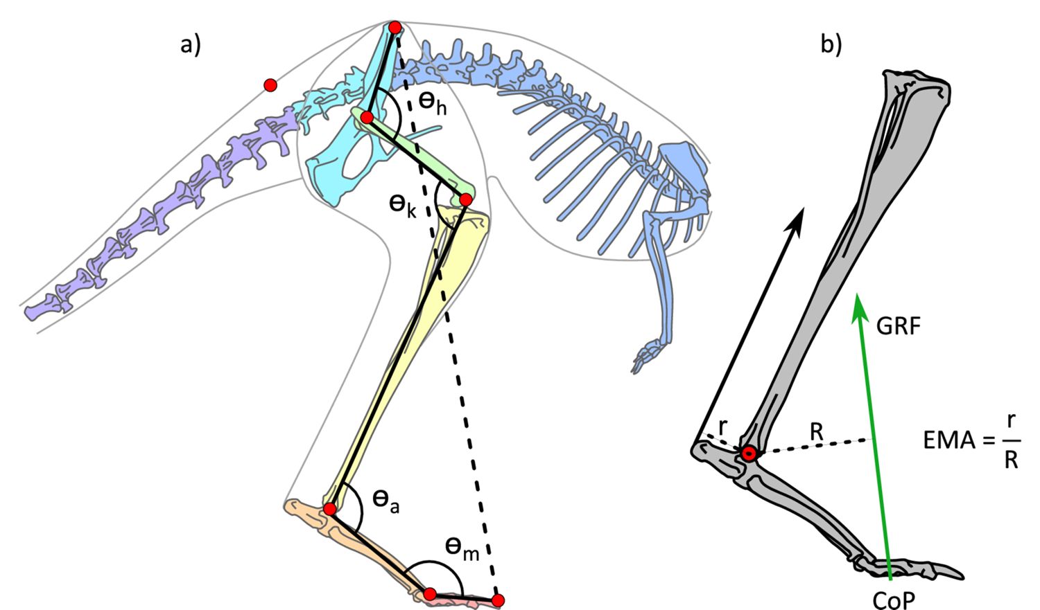
Illustration of the kangaroo model and moment arms for the ankle.
(a) Illustration of the kangaroo model. Total leg length was calculated as the sum of the segment lengths (solid black lines) in the hindlimb and compared to the pelvis-to-toe distance (dashed line) to calculate the crouch factor. Joint angles were determined for the hip, h, knee, k, ankle, a, and metatarsophalangeal, m, joints. The model markers (red circles) indicate the position of the reflective markers placed on the kangaroos in the experimental trials and were used to characterise the movement of segments in the musculoskeletal model. (b) Illustration of ankle effective mechanical advantage, EMA, muscle moment arm, r, and external moment arm, R, as the perpendicular distance to the Achilles tendon line of action and ground reaction force (GRF) vector, respectively. The centre of pressure (CoP) was tracked in the fore-aft direction.
Figure 1—figure supplement 1

Distribution of trial speeds and number of trials (n) per kangaroo (6.25±5.02 trials per kangaroo).
Figure 1—video 1
A red kangaroo hopping on the force plate during data collection.
Figure 1—video 2
Driving the musculoskeletal model with a recorded hopping trial.
The gastrocnemius and plantaris muscle-tendon unit (Achilles) is shown in blue. The GRF appears in green. Markers associating the recorded kangaroos with the model are in pink.
Figure 2 with 3 supplements

Horizontal fore-aft (dashed lines) and vertical (solid lines) components of the ground reaction force (GRF) (a) coloured by body mass subsets (small 17.6±2.96 kg, medium 21.5±0.74 kg, large 24.0±1.46 kg) and (b) coloured by speed subsets (slow 2.52±0.25 ms–1, medium 3.11±0.16 ms–1, fast 3.79±0.27 ms–1).
In (a) and (b), the medial-lateral component of the GRF is not shown as it remained close to zero, as expected for animals moving in a straight-line path. Lower panels show average time-varying effective mechanical advantage (EMA) for the ankle joint subset by (c) body mass and (d) speed.
Figure 2—figure supplement 1

Kinematics of the stride with speed and stance.
(a) Mean vertical and horizontal components of whole body acceleration for kangaroos in the slow, medium, and fast subsets (respectively: 2.52±0.25 ms–1, 3.11±0.16 ms–1, 3.79±0.27 ms–1). (b) Ground contact duration across hopping speeds from current study (black circles) and for red kangaroos reported in Kram and Dawson, 1998 (red circles). Regression equation: tc = 0.342 speed-0.477 where tc is contact duration and s is hopping speed. (c) Relationship between stride length and speed, and (d) stride frequency and speed.
Figure 2—figure supplement 2

Vertical ground reaction force with mass and speed.
(a) Relationship between peak vertical ground reaction force (GRF) as a multiple of body weight (BW) with body mass and (b) with speed.
Dotted line is insignificant and solid line is significant, see Appendix 1—table 2 for interaction.
Figure 2—figure supplement 3

Peak vertical ground reaction force (GRF) plotted against tendon stress (Β=0.080, SE = 0.009, p<0.001, R2=0.486).
Figure 3 with 2 supplements

Average time-varying crouch factor (see Figure 1a) of the kangaroo hindlimb grouped by (a) body mass and (c) speed.
Position of the limb segments during % stance intervals (b). Average time-varying joint angles for the hip (solid lines) and knee (dashed lines) displayed for kangaroos grouped by (d) body mass and (e) speed. Average time-varying joint angles for the ankle (solid lines) and metatarsophalangeal (MTP) joints (dashed lines) displayed for kangaroos grouped by (f) body mass and (g) speed. For (f–g), increased plantarflexion represents a decrease in joint flexion, while increased dorsiflexion represents increased flexion of the joint. Body mass subsets: small 17.6±2.96 kg, medium 21.5±0.74 kg, large 24.0±1.46 kg. Speed subsets: slow 2.52±0.25 ms–1, medium 3.11±0.16 ms–1, fast 3.79±0.27 ms–1.
Figure 3—figure supplement 1

Average time-varying gastrocnemius and plantaris muscle moment arm, r, grouped by (a) body mass and (b) speed; external moment arm to the ankle, R, grouped by (c) body mass, and (d) speed.
Vertical displacement of the ankle marker from the ground throughout stance grouped by (e) body mass and (f) speed. Ankle angles and corresponding r arm length (g). Length of the r and R moment arms at midstance at different speeds (h). Body mass subsets: small 17.6±2.96 kg, medium 21.5±0.74 kg, large 24.0±1.46 kg. Speed subsets: slow 2.52±0.25 ms–1, medium 3.11±0.16 ms–1, fast 3.79±0.27 ms–1.
Figure 3—figure supplement 2

Average time-varying net joint moments (dimensionless, as moments were divided by body weight * leg length) for the hip (solid lines) and knee (dotted lines) displayed for kangaroos grouped by (a) body mass and (b) speed.
Average time-varying net joint moments (dimensionless) for the ankle (solid lines) and metatarsophalangeal (MTP; dotted lines) joints displayed for kangaroos grouped by (c) body mass and (d) speed. Data for tammar wallabies was also included (McGowan et al., 2005) in green. Peak ankle moment occurred at 47.37±4.91% of the stance phase. Positive values represent extensor moments and negative values represent flexor moments. Body mass subsets: small 17.6±2.96 kg, medium 21.5±0.74 kg, large 24.0±1.46 kg. Speed subsets: slow 2.52±0.25 ms–1, medium 3.11±0.16 ms–1, fast 3.79±0.27 ms–1.
Figure 4

EMA with stress and mass.
(a) Relationship between ankle effective mechanical advantage, EMA, at midstance and Achilles tendon stress (stress = 11.6 EMA-1.04, R2=0.593) (black), with other mammals (green). (b) Scaling of mean ankle EMA at midstance for each individual kangaroo against body mass (black), with data for a wider range of macropods (purple) (Bennett and Taylor, 1995), and other mammals (green, EMA = 0.269 M0.259, shaded area 95% confidence interval) (Biewener, 1990) shown.
Figure 5

Time-varying joint powers.
Average time-varying joint powers for the hip (a, b), knee (c, d), ankle (e, f), and MTP (g, h) displayed for kangaroos grouped by body mass (a, c, e, g) and speed (b, d, f, h). Power in all panels is set to the same scale. Body mass subsets: small 17.6±2.96 kg, medium 21.5±0.74 kg, large 24.0±1.46 kg. Speed subsets: slow 2.52±0.25 ms–1, medium 3.11±0.16 ms–1, fast 3.79±0.27 ms–1.
Figure 6 with 3 supplements

Variation with speed of (a) positive and negative ankle work, and (b) net ankle work per hop.
Figure 6—figure supplement 1

Positive (purple) and negative (green) joint work over stance for the hip, knee, ankle, and metatarsophalangeal (MTP) plotted against body mass (a, c, e, g) and speed (b, d, f, h).
Solid lines represent significant trends, dotted lines are not significant (see Appendix 1—table 6).
Figure 6—figure supplement 2

Net joint work for the hip, knee, ankle, and metatarsophalangeal (MTP) joint over stance plotted against body mass (a, c, e, g) and speed (b, d, f, h).
Solid lines represent significant trends, dotted lines are not significant (see Appendix 1—table 6).
Figure 6—figure supplement 3

Ankle work with EMA at midstance.
Negative (a) (Β=−3.04, SE=0.75, p<0.001, R2=0.155), positive (b) (Β=−7.42, SE=0.61, p<0.001, R2=0.622), and net ankle work (c) (Β=−4.37, SE=0.84, p<0.001, R2=0.230) plotted against effective mechanical advantage (EMA) at 50% of stance.
Figure 7

How the relationship between posture and speed is proposed to change tendon stress.
Forces are not to scale and joint angles are exaggerated for illustrative clarity. A slow hop (left panel) compared to a fast hop (right panel). The increase in ground reaction force (GRF) with speed, while a more crouched posture changes the muscle moment arm, r, and external moment arm, R, which allows the ankle to do more negative work (storing elastic potential energy in the tendons due to greater tendon stresses), without increasing net work, and thereby metabolic cost. Ankle moment was calculated by OpenSim and includes inertial terms.
Tables
Appendix 1—table 1
Stride parameter multiple linear regression results as slopes, standard errors, and p-values.
Models with a significant interaction are displayed in full, and as a simplified model without the interaction term included (marked *). The fit of the model is represented by R2 and relationships are considered significant at p<0.05.
| Interaction | Body mass | Speed | R2 | |||||||
|---|---|---|---|---|---|---|---|---|---|---|
| β | SE | P | β | SE | P | β | SE | P | ||
| Maximum vertical acceleration (ms–2) | –1.19 | 0.567 | 0.038 | 2.72 | 1.64 | 0.100 | 32.5 | 12.5 | 0.011 | 0.190 |
| Maximum vertical acceleration (ms–2)* | –0.673 | 0.294 | 0.024 | 6.32 | 1.60 | 0.000 | 0.152 | |||
| Minimum vertical acceleration (ms–2) | 0.221 | 0.208 | 0.290 | –0.268 | 1.13 | 0.814 | 0.012 | |||
| Maximum horizontal acceleration (ms–2) | –0.036 | 0.296 | 0.903 | 0.159 | 1.61 | 0.922 | 0.000 | |||
| Minimum horizontal acceleration (ms–2) | 0.407 | 0.370 | 0.275 | –6.05 | 2.02 | 0.003 | 0.087 | |||
| Contact duration (ms) | 2.87 | 0.393 | 0.000 | –34.2 | 2.12 | 0.000 | 0.735 | |||
| Stride length (m) | 0.014 | 0.004 | 0.001 | 0.376 | 0.020 | 0.000 | 0.815 | |||
| Stride frequency (Hz) | 0.022 | 0.008 | 0.007 | –0.082 | 0.023 | 0.001 | –0.392 | 0.180 | 0.032 | 0.303 |
| Stride frequency (Hz)* | –0.019 | 0.004 | 0.000 | 0.102 | 0.023 | 0.000 | 0.245 | |||
Appendix 1—table 2
Ground reaction force and centre of pressure (CoP) multiple linear regression results as slopes, standard errors, and p-values.
Models with a significant interaction are displayed in full, and as a simplified model without the interaction term included (marked *). The fit of the model is represented by R2 and relationships are considered significant at p<0.05.
| Interaction | Body mass | Speed | R2 | |||||||
|---|---|---|---|---|---|---|---|---|---|---|
| β | SE | P | β | SE | P | β | SE | P | ||
| Normalised peak GRF (BW) | –0.055 | 0.024 | 0.026 | 0.111 | 0.070 | 0.117 | 1.34 | 0.535 | 0.014 | 0.172 |
| Normalised peak GRF (BW)* | –0.045 | 0.013 | 0.001 | 0.142 | 0.068 | 0.040 | 0.128 | |||
| Peak vertical GRF (N) | –11.5 | 5.31 | 0.032 | 47.9 | 15.4 | 0.002 | 281 | 117 | 0.019 | 0.332 |
| Peak vertical GRF (N)* | 15.0 | 2.76 | 0.000 | 28.4 | 14.9 | 0.060 | 0.299 | |||
| Peak braking GRF (N) | 4.87 | 2.04 | 0.019 | –14.8 | 5.90 | 0.014 | –130 | 45.0 | 0.005 | 0.218 |
| Peak braking GRF (N)* | –0.917 | 1.07 | 0.392 | –23.2 | 5.76 | 0.000 | 0.172 | |||
| Peak propulsive GRF (N) | 2.03 | 0.818 | 0.015 | 21.5 | 4.42 | 0.000 | 0.285 | |||
| CoP location at midstance (mm) | –0.123 | 1.54 | 0.937 | –15.2 | 8.34 | 0.071 | 0.036 | |||
| CoP location at midstance corrected for phalanx size (mm) | –0.437 | 17.0 | 0.980 | –62.7 | 91.9 | 0.497 | 0.005 | |||
Appendix 1—table 3
Crouch factor (CF) and kinematics multiple linear regression results as slopes, standard errors, and p-values.
Models with a significant interaction are displayed in full, and as a simplified model without the interaction term included (marked *). The fit of the model is represented by R2 and relationships are considered significant at p<0.05.
| Interaction | Body mass | Speed | R2 | |||||||
|---|---|---|---|---|---|---|---|---|---|---|
| β | SE | P | β | SE | P | β | SE | P | ||
| Maximum CF | –2.19 | 1.07 | 0.043 | –15.8 | 5.74 | 0.007 | 0.122 | |||
| Minimum CF | –2.45 | 0.885 | 0.007 | –1.53 | 4.76 | 0.749 | 0.064 | |||
| Change in CF | 0.256 | 0.661 | 0.699 | –14.2 | 3.55 | 0.000 | 0.129 | |||
| Pelvis pitch ROM (deg) | 0.935 | 0.298 | 0.002 | –2.60 | 0.862 | 0.003 | –19.9 | 6.58 | 0.003 | 0.100 |
| Pelvis pitch ROM (deg)* | 0.066 | 0.159 | 0.677 | 0.534 | 0.858 | 0.535 | 0.008 | |||
| Hip ROM (deg) | –0.488 | 0.212 | 0.024 | 0.490 | 1.15 | 0.670 | 0.052 | |||
| Minimum hip flexion (deg) | –0.655 | 0.315 | 0.040 | 0.703 | 1.70 | 0.681 | 0.043 | |||
| Maximum hip flexion (deg) | –0.167 | 0.260 | 0.520 | 0.213 | 1.40 | 0.880 | 0.004 | |||
| Knee ROM (deg) | –1.31 | 0.520 | 0.013 | 2.88 | 1.50 | 0.058 | 28.6 | 11.5 | 0.014 | 0.154 |
| Knee ROM (deg)* | –0.850 | 0.272 | 0.002 | –0.120 | 1.47 | 0.935 | 0.098 | |||
| Minimum knee flexion (deg) | –1.72 | 0.649 | 0.010 | 3.76 | 1.88 | 0.048 | 39.5 | 14.3 | 0.007 | 0.162 |
| Minimum knee flexion (deg)* | –1.13 | 0.34 | 0.001 | 1.95 | 1.84 | 0.294 | 0.101 | |||
| Maximum knee flexion (deg) | –0.277 | 0.265 | 0.299 | 2.07 | 1.43 | 0.152 | 0.026 | |||
| Ankle ROM (deg) | 1.02 | 0.166 | 0.000 | 1.63 | 0.899 | 0.073 | 0.339 | |||
| Peak ankle plantarflexion (deg) | –0.173 | 0.240 | 0.474 | –3.87 | 1.30 | 0.004 | 0.104 | |||
| Peak ankle dorsiflexion (deg) | –1.19 | 0.198 | 0.000 | –5.49 | 1.07 | 0.000 | 0.466 | |||
| MTP ROM (deg) | –0.098 | 0.259 | 0.707 | 7.16 | 1.40 | 0.000 | 0.219 | |||
| Peak MTP plantarflexion (deg) | 0.875 | 0.306 | 0.005 | 5.64 | 1.65 | 0.001 | 0.216 | |||
| Peak MTP dorsiflexion (deg) | 0.973 | 0.221 | 0.000 | –1.52 | 1.20 | 0.205 | 0.166 | |||
Appendix 1—table 4
Multiple linear regression results of dimensionless peak joint moments as slopes, standard errors, and p-values.
Models with a significant interaction are displayed in full, and as a simplified model without the interaction term included (marked *). The fit of the model is represented by R2 and relationships are considered significant at p<0.05.
| Interaction | Body mass | Speed | R2 | |||||||
|---|---|---|---|---|---|---|---|---|---|---|
| β | SE | P | β | SE | P | β | SE | P | ||
| Hip extensor moment | –0.020 | 0.006 | 0.001 | 0.049 | 0.018 | 0.007 | 0.525 | 0.136 | 0.000 | 0.268 |
| Hip extensor moment* | –0.009 | 0.003 | 0.010 | 0.079 | 0.018 | 0.000 | 0.184 | |||
| Knee extensor moment | 0.000 | 0.001 | 0.766 | 0.003 | 0.008 | 0.721 | 0.003 | |||
| Knee flexor moment | 0.020 | 0.005 | 0.000 | –0.048 | 0.015 | 0.002 | –0.487 | 0.116 | 0.000 | 0.264 |
| Knee flexor moment* | 0.008 | 0.003 | 0.007 | –0.060 | 0.015 | 0.000 | 0.158 | |||
| Ankle extensor moment | –0.004 | 0.004 | 0.256 | 0.043 | 0.020 | 0.036 | 0.048 | |||
| MTP extensor moment | –0.001 | 0.002 | 0.767 | 0.000 | 0.013 | 0.986 | 0.001 | |||
Appendix 1—table 5
Tendon stress and effective mechanical advantage (EMA) multiple linear regression results as slopes, standard errors, and p-values.
Models with a significant interaction are displayed in full, and as a simplified model without the interaction term included (marked *). The fit of the model is represented by R2 and relationships are considered significant at p<0.05.
| Interaction | Body mass | Speed | R2 | |||||||
|---|---|---|---|---|---|---|---|---|---|---|
| β | SE | P | β | SE | P | β | SE | P | ||
| r at midstance (mm) | –0.063 | 0.088 | 0.477 | –1.88 | 0.474 | 0.000 | 0.173 | |||
| R at midstance (mm) | 3.49 | 1.03 | 0.001 | –0.93 | 5.59 | 0.869 | 0.117 | |||
| EMA at midstance | –6.64 | 1.98 | 0.001 | –11.0 | 10.7 | 0.310 | 0.142 | |||
| Peak tendon stress (MPa) | 1.03 | 0.385 | 0.008 | 5.61 | 2.08 | 0.008 | 0.168 | |||
| Normalised peak tendon stress | –0.048 | 0.018 | 0.008 | 0.258 | 0.096 | 0.008 | 0.107 | |||
| Peak tendon stress timing % stance | –0.151 | 0.154 | 0.328 | –3.13 | 0.831 | 0.000 | 0.159 | |||
| Ankle height from ground (mm) | –0.298 | 0.706 | 0.674 | –23.0 | 3.81 | 0.000 | 0.295 | |||
Appendix 1—table 6
Joint net positive, negative and net work simple linear regression (lm(joint work ~mass), lm(joint work ~speed)) results as slopes, standard errors, and p-values.
Work is normalised by body mass (BM). The fit of the model is represented by R2 and relationships are considered significant at p<0.05.
| Body mass | Speed | |||||||
|---|---|---|---|---|---|---|---|---|
| β | SE | P | R2 | β | SE | P | R2 | |
| Hip pos | –0.010 | 0.008 | 0.238 | 0.014 | 0.030 | 0.044 | 0.497 | 0.005 |
| Hip neg | –0.027 | 0.005 | 0.000 | 0.225 | –0.058 | 0.031 | 0.066 | 0.034 |
| Hip net | 0.018 | 0.007 | 0.018 | 0.055 | 0.087 | 0.041 | 0.034 | 0.045 |
| Knee pos | –0.021 | 0.011 | 0.052 | 0.038 | 0.145 | 0.057 | 0.013 | 0.061 |
| Knee neg | –0.004 | 0.004 | 0.267 | 0.013 | –0.046 | 0.020 | 0.026 | 0.050 |
| Knee net | –0.017 | 0.012 | 0.169 | 0.019 | 0.191 | 0.064 | 0.003 | 0.084 |
| Ankle pos | 0.059 | 0.019 | 0.003 | 0.087 | 0.478 | 0.097 | 0.000 | 0.197 |
| Ankle neg | 0.022 | 0.017 | 0.200 | 0.017 | 0.321 | 0.087 | 0.000 | 0.122 |
| Ankle net | 0.037 | 0.017 | 0.037 | 0.044 | 0.156 | 0.095 | 0.102 | 0.027 |
| MTP pos | –0.003 | 0.008 | 0.743 | 0.001 | –0.046 | 0.043 | 0.286 | 0.012 |
| MTP neg | 0.023 | 0.014 | 0.089 | 0.029 | 0.149 | 0.073 | 0.044 | 0.041 |
| MTP net | –0.026 | 0.012 | 0.035 | 0.045 | –0.194 | 0.064 | 0.003 | 0.086 |
Appendix 1—table 7
Positive, negative and net joint work multiple linear regression results as slopes, standard errors, and p-values.
Work is normalised by body mass (BM). Models with a significant interaction are displayed in full, and as a simplified model without the interaction term included (marked *). The fit of the model is represented by R2 and relationships are considered significant at p<0.05.
| Joint work (Jkg–1 BM) | Interaction | Body mass | Speed | R2 | ||||||
|---|---|---|---|---|---|---|---|---|---|---|
| β | SE | P | β | SE | P | β | SE | P | ||
| Hip positive | 0.046 | 0.045 | 0.307 | –0.012 | 0.008 | 0.161 | 0.025 | |||
| Hip negative | –0.021 | 0.029 | 0.472 | –0.026 | 0.005 | 0.000 | 0.229 | |||
| Hip net | 0.067 | 0.042 | 0.110 | 0.015 | 0.008 | 0.058 | 0.080 | |||
| Knee positive | –0.072 | 0.020 | 0.000 | 1.766 | 0.431 | 0.000 | 0.175 | 0.057 | 0.003 | 0.241 |
| Knee positive* | 0.187 | 0.057 | 0.002 | –0.030 | 0.011 | 0.006 | 0.133 | |||
| Knee negative | –0.043 | 0.021 | 0.045 | –0.002 | 0.004 | 0.570 | 0.053 | |||
| Knee net | –0.073 | 0.022 | 0.002 | 1.818 | 0.491 | 0.000 | 0.179 | 0.064 | 0.007 | 0.219 |
| Knee net* | 0.230 | 0.064 | 0.001 | –0.028 | 0.012 | 0.021 | 0.133 | |||
| Ankle positive | 0.424 | 0.099 | 0.000 | 0.039 | 0.018 | 0.038 | 0.232 | |||
| Ankle negative | –0.080 | 0.032 | 0.015 | 2.052 | 0.707 | 0.005 | 0.234 | 0.093 | 0.013 | 0.176 |
| Ankle negative* | 0.311 | 0.091 | 0.001 | 0.007 | 0.017 | 0.671 | 0.123 | |||
| Ankle net | 0.122 | 0.033 | 0.000 | –2.551 | 0.732 | 0.001 | –0.315 | 0.096 | 0.001 | 0.173 |
| Ankle net* | 0.112 | 0.097 | 0.250 | 0.031 | 0.018 | 0.084 | 0.057 | |||
| MTP positive | –0.045 | 0.044 | 0.312 | 0.000 | 0.008 | 0.956 | 0.012 | |||
| MTP negative | 0.125 | 0.075 | 0.101 | 0.017 | 0.014 | 0.217 | 0.056 | |||
| MTP net | –0.170 | 0.066 | 0.011 | –0.018 | 0.012 | 0.149 | 0.106 | |||
Appendix 1—table 8
The mean and standard deviation of joint work for all trials.
Positive, negative, and net work is presented for each joint.
| Joint work (Jkg–1 BM) | Mean | SD |
|---|---|---|
| Hip positive | 0.38 | 0.246 |
| Hip negative | 0.187 | 0.178 |
| Hip net | 0.193 | 0.235 |
| Knee positive | 0.432 | 0.334 |
| Knee negative | 0.104 | 0.117 |
| Knee net | 0.328 | 0.375 |
| Ankle positive | 1.99 | 0.613 |
| Ankle negative | 1.324 | 0.525 |
| Ankle net | 0.666 | 0.542 |
| MTP positive | 0.294 | 0.242 |
| MTP negative | 0.652 | 0.42 |
| MTP net | –0.358 | 0.377 |
Additional files
Download links
A two-part list of links to download the article, or parts of the article, in various formats.
Downloads (link to download the article as PDF)
Open citations (links to open the citations from this article in various online reference manager services)
Cite this article (links to download the citations from this article in formats compatible with various reference manager tools)
Postural adaptations may contribute to the unique locomotor energetics seen in hopping kangaroos
eLife 13:RP96437.
https://doi.org/10.7554/eLife.96437.3


