Homeostatic synaptic normalization optimizes learning in network models of neural population codes
Figures
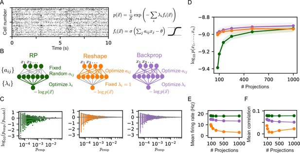
Reshaped Random Projections (RP) models outperform RP models.
(A) A short segment of the spiking activity of 100 cortical neurons used for the analysis and comparison of different statistical models of population activity (see Materials and methods). (B) Schematics of the neural circuits that implement the different RP models we compared: The ‘standard’ RP model, where the coefficients that define the projections are randomly selected and fixed whereas the factors are learned (see text). The Reshaped RP model, where the coefficients that define the projections are tuned and the factors s are fixed. The backpropagation model, where we tune both the s and s. (C) The predicted probability of individual populations’ activity patterns as a function of the observed probability for RP, Reshaped, and backpropagation models. Gray funnels denote 99% confidence interval. (D) Average performance of models of the three classes is shown as a function of the number of projections, measured by log-likelihood, over 100 sets of randomly selected groups of 50 neurons. Reshaped models outperform RP models and are on par with backpropagation; the shaded area denotes the standard error over 100 models. (E–F) Mean firing rates of projection neurons and mean correlation between projections. Reshaped models show lower correlations and lower firing rates compared to RP and backpropagation models. Standard errors are smaller than marker’s size, hence invisible.
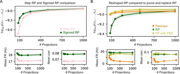
Comparison of different Random Projections (RP) model variants .
(A) Average performance measured by log-likelihood (top), projections mean firing rates (bottom left), and mean correlation between projections (bottom right) of step and sigmoid RP models as a function of the number of projections. Sigmoid RP models outperform step RP models, and show higher mean firing rates and correlations. (B) Average performance measured by log-likelihood (top), projections mean firing rates (bottom left), and mean correlation between projections (bottom right) of RP and Reshaped RP models compared to RP models after pruning and replacement (P&R). RP models after P&R are very accurate even though a small number of parameters is optimized at each iteration. In all panels shaded area denotes standard error over 100 models.
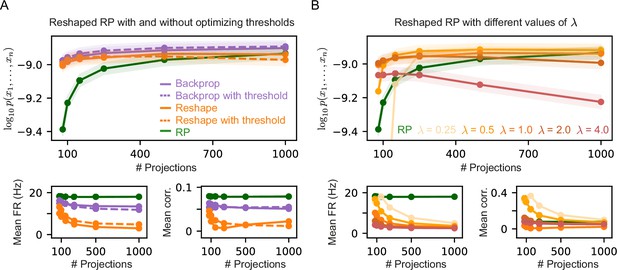
Comparison of different Reshaped Random Projections (RP) model variants.
(A) Average performance measured by log-likelihood (top), projections mean firing rates (bottom left), and mean correlation between projections (bottom right) of Reshaped RP and backpropagation models with optimized threshold , compared to models with fixed thresholds. Threshold optimization has little to non effect on the models performance, mean firing rates, and mean correlations. (B) Average performance measured by log-likelihood (top), projections mean firing rates (bottom left), and mean correlation between projections (bottom right) of Reshaped RP models with different fixed values of λ. Models with higher values of λ show lower mean firing rates and mean correlation values. In all panels, shaded areas denote standard error over 100 models.
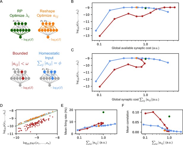
Reshaped RP models that use homeostatic synaptic normalization outperform RP models and bounded RP models.
(A) Schematic drawing of the different models we studied: standard RP model, unconstrained reshaped model, and two types of constrained reshaped models: Bounded models in which each synapse separately obeys during learning, and normalized input reshaped models, where we fix the total synaptic weight of incoming synapses . (B) The mean log-likelihood of the models is shown as a function of the total available budget. The normalized input reshaped RP models give optimal results for a wide range of values of available synaptic budget, outperforming the bounded models and the RP model. (C) The mean log-likelihood of the models is shown as a function of the total used budget. Aside from the bounded models, all other models are the same as in (B) by construction. For high available budget values, bounded models show better performance while utilizing a lower synaptic budget, similar to the unconstrained reshape model. (D) Comparison of the performance of 100 individual examples of each model class and their corresponding RP models, where all models relied on the same set of initial projections. Normalized input models outperformed the RP models in all cases (all points are above the diagonal), while all bounded models were worse (points below the diagonal). (E–F) The mean correlation and firing rates of projections as a function of the model’s cost. Normalized reshape models show low correlations and mean firing rates, similar to unconstrained reshaped models. Note that in panels B, C, E, and F, the standard errors are smaller than the marker size, and are therefore invisible.

Homeostatic models are superior to Reshaped RP models for every choice of .
Mean log-likelihood of homeostatic and reshaped RP models with different fixed values of , as a function total used synaptic cost. For every choice of , there exists a homeostatic model which is more efficient and preforms similarly or better than the corresponding reshaped RP model. Standard error is smaller than marker size, hence cannot be seen.
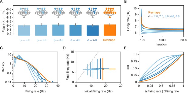
Homeostatic models’ performance and firing rates.
(A) Likelihood values of the different homeostatic models we consider here; Error bars denote standard error over 100 different models. (B) Projections’ mean firing rates during reshaping; Standard error is smaller than marker size, hence cannot be seen (C) A histogram of the projections’ firing rates of unconstrained models and different homeostatic input models. (D) Projections’ mean firing rates after reshaping vs. the projection’s initial firing rate, for different homeostatic models and unconstrained model; Error bars denote standard deviation over 100 different models. (E) The cumulative density function of the projections’ firing rate relative change during reshape, .
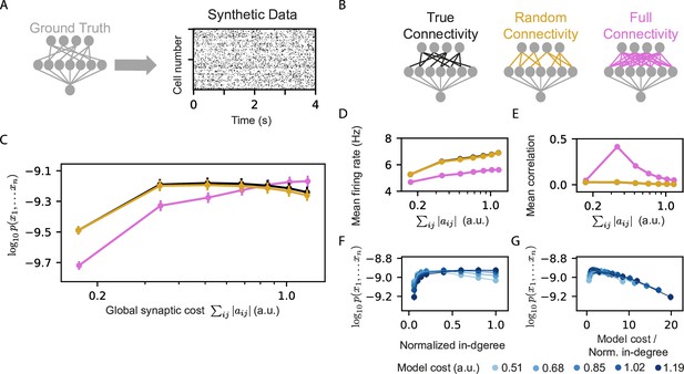
Models that rely on projections that use random connectivity show similar performance to models that use the correct connectivity.
(A) Synthetic population activity data is sampled from an RP model with known connectivity (i.e. the ‘ground truth’ model; see Materials and methods). (B) Homeostatic Reshaped random projections models that differ in their connectivity are learned to fit the synthetic data. The ‘True connectivity’ model uses projections whose connectivity is identical to the ‘ground truth’ model. The ‘Random connectivity’ model uses projections that are randomly sampled using sparse random connectivity. The ‘Full connectivity’ model is a homeostatic reshaped model that uses projections with full connectivity. (C) The mean log-likelihood of the models is shown as a function of the model’s cost. The true connectivity model is only slightly better than the random connectivity model, with both outperforming the full connectivity model for low model budget values. (D) The firing rates of the projection neurons, shown as a function of the model cost. (E) The mean correlation between the activity of the projection neurons, shown as a function of the model cost. We note that true and random connectivity models are indistinguishable. (F) The performance of homeostatic reshaped RP models, shown as a function of their normalized in-degree of the projections (0–disconnected, 1–fully connected), for different normalization values, shown by the model’s synaptic cost. (G) The performance of the homeostatic Reshaped RP models, shown as a function of the synaptic cost normalized by the in-degree of the projections. Curves of different cost values coincide, suggesting a fixed optimal cost/activity ratio. Note that in panels D-G the standard errors over 100 models are smaller than the size of markers and are, therefore, invisible.
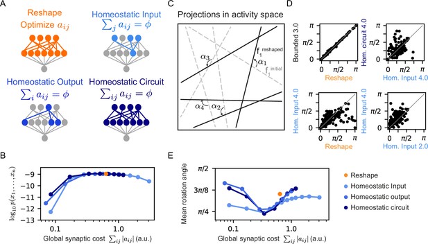
Different homeostatic synaptic normalization mechanisms result in similar model behavior, for a wide range of random projection parameters.
(A) Schematic drawings of the different homeostatic models we compared: Homeostatic input models in which we fixed the total synaptic weight of the incoming synapses ; Homeostatic output models in which we fixed the total synaptic weight of the outgoing synapses ; and Homeostatic circuit models in which we fixed the total synaptic weight of the whole synaptic circuit . (B) The mean log-likelihood of models, shown as a function of the total used synaptic cost. All three homeostatic model variants show similar behavior. (C) Schematic drawing of how projections rotate during reshaping: starting from the initial projections (grey lines), they rotate to their reshaped orientation (black lines) by angle . (D) Rotation angles after reshaping, shown for different pairs of models. All four panels show models that initialized with the same set of projections. The different labels specify the constraint type and strength, namely, the specific value of and . (E) The mean rotation angle of the projections due to reshaping, shown as a function of the model synaptic budget.
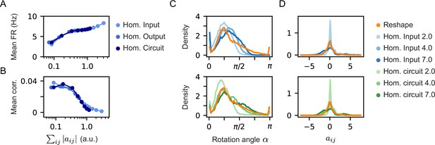
Homeostatic model variants show similar firing rates and correlation, but different rotation angles and distribution of weights.
(A) and (B) Mean correlation between the projection neurons and mean firing rates as a function of the model cost of the three different homeostatic models we compared. All three homeostatic models show a similar behavior. Note that the standard errors over 100 models are smaller than the marker’s size and are, therefore, invisible. (C) Histograms of rotation angles of the projections after learning in the case of the unconstrained reshape models and different homeostatic input (top) and homeostatic circuit (bottom) models. (D) Histograms of weight distribution after learning in the case of the unconstrained reshape models and different homeostatic input (top) and homeostatic circuit (bottom) models. The legend specifies the constraint type and strength, namely, the specific value of Φ.


