A dynamic generative model can extract interpretable oscillatory components from multichannel neurophysiological recordings
- Department of Anesthesiology, Perioperative and Pain Medicine, Stanford University, United States
- Department of Psychology, Stanford University, United States
- Department of Bioengineering, Stanford University, United States
Figures
Figure 1
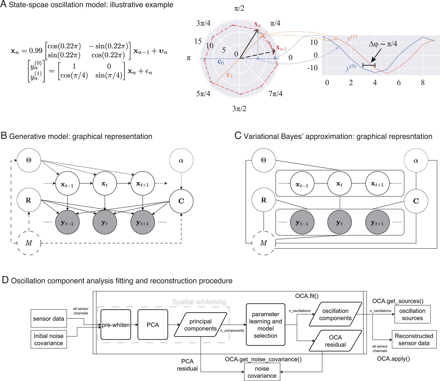
From state-space oscillator model to oscillation component decomposition.
(A) An illustrative example of a multichannel state-space oscillation model: a single oscillation realized as an analytic signal is measured as two different projections having radian phase difference. (B) Graphical representation of the probabilistic generative model describing the oscillations as dynamic processes that undergo mixing at the sensors and that are observed with additive Gaussian noise. (C) Graphical representation of the variational Bayes approximation that allows iterative closed-form inference. (D) Oscillation component analysis fitting and reconstruction pipeline for experimentally recorded neurophysiological data. The pipeline exposes a number of methods for ease of analysis, that is, for fitting the oscillation component analysis (OCA) hyperparameters fit () method, which accepts the sensor recordings and an initial sensor noise covariance matrix as input, extracting the oscillation time courses get_sources(), reconstructing a multichannel signal from any arbitrary subset of oscillation components, apply(), getting a final noise covariance estimate from the residuals of OCA fitting, get_noise_covariance() method, etc.
Figure 2
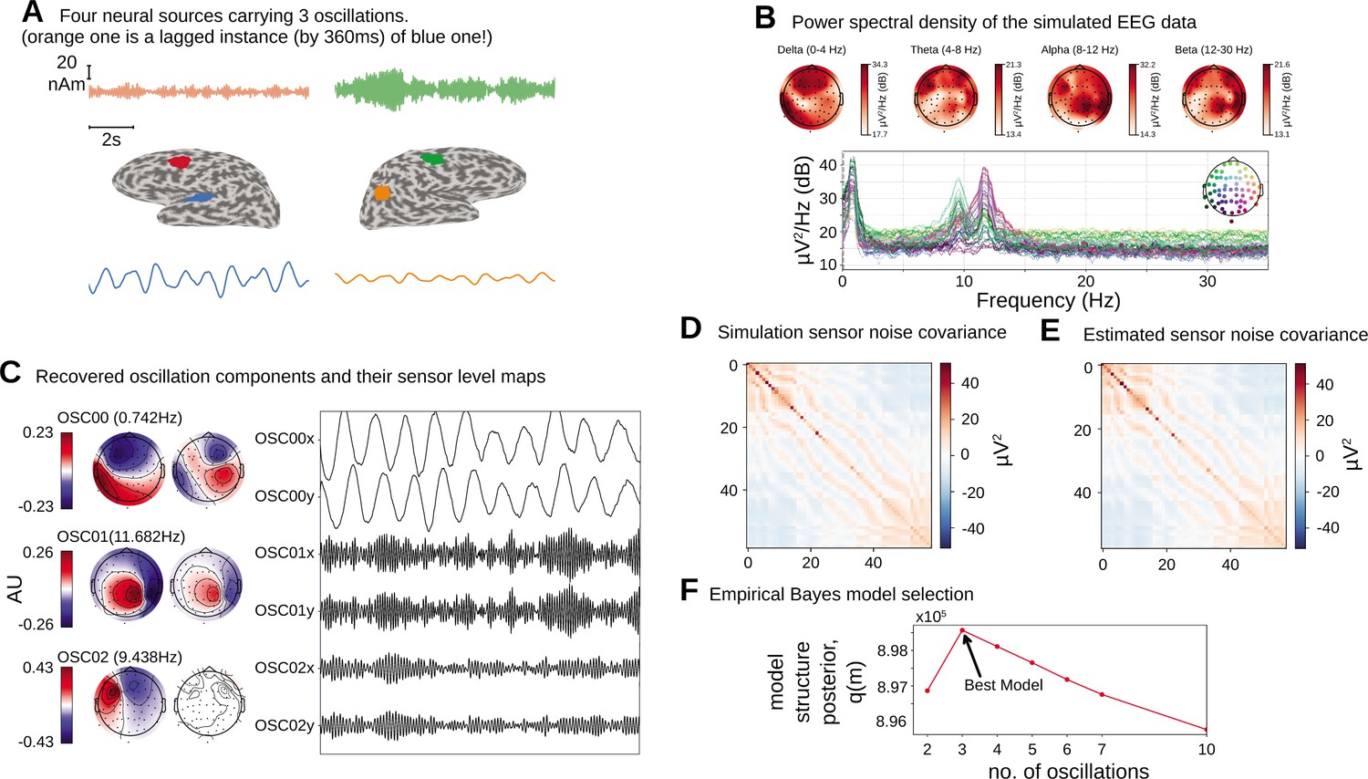
Simulation study.
(A).Four neural sources carrying three oscillations, where the orange time course is a lagged instance of blue time course, red and green time courses are independent. (B) Power spectral density of the simulated electroencephalogram (EEG) recording and power distribution over the EEG sensors in different frequency bands. (C) Recovered oscillation components and their sensor-level maps. (D) Sensor noise covariance for the simulation. (E) Estimated sensor noise covariance matrix. (F) Model structure selection via model structure posterior .
Figure 3
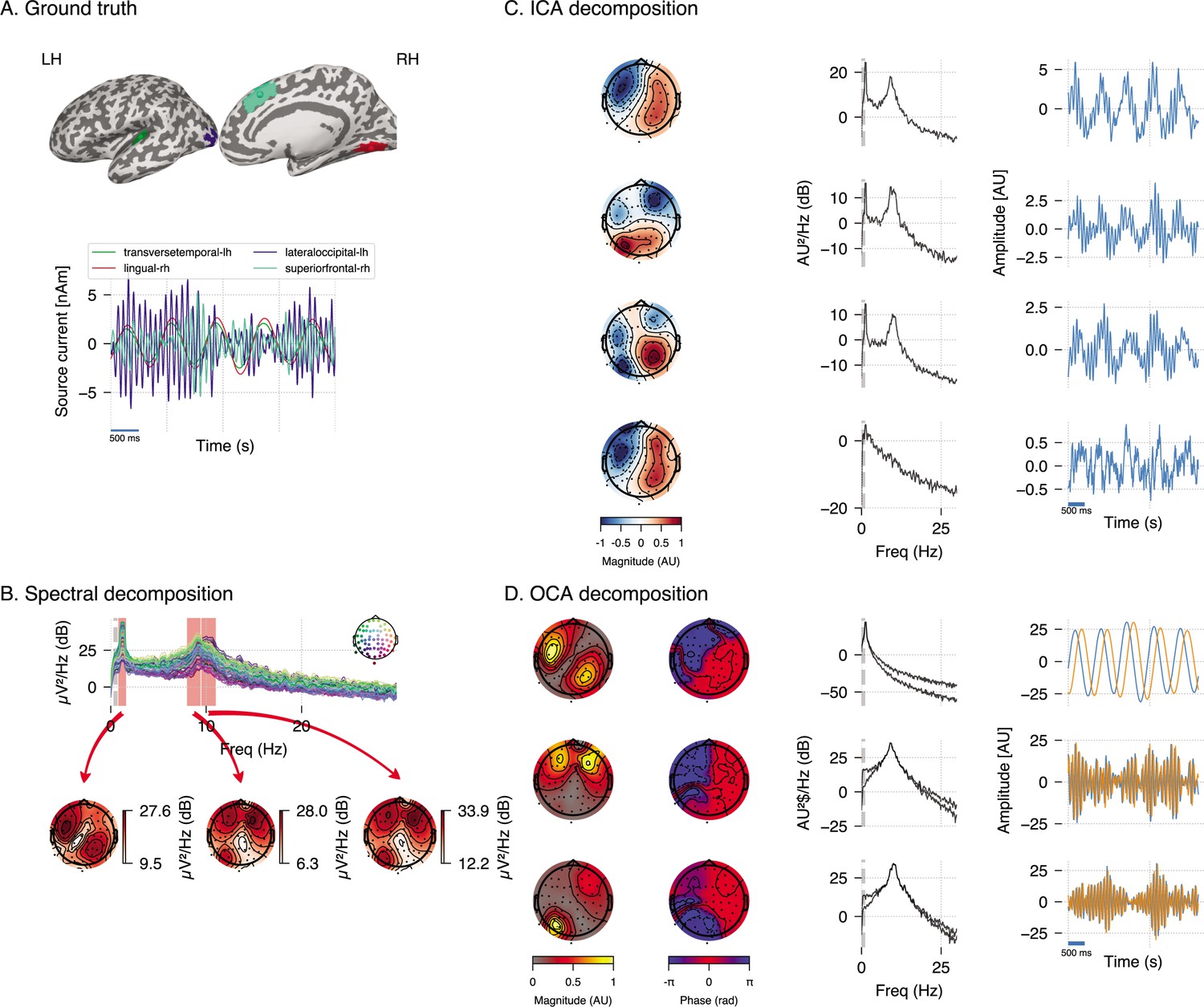
Simulation study (extended).
(A) Four neural sources carrying three oscillations, similar to Figure 2. (B) Power spectral density of the simulated electroencephalogram (EEG) recording and power distribution over the EEG sensors in the frequency bands (red overlay) around visually identifiable peaks. (C) Recovered independent component analysis (ICA) components (left, middle, and right columns show topographic maps, power spectrum density, and time courses, respectively). (D) Recovered oscillation component analysis (OCA) components (the topographic maps show the magnitude [left] and phase [right], while line plots show power spectrum density [left] and time courses [right], respectively).
Figure 4
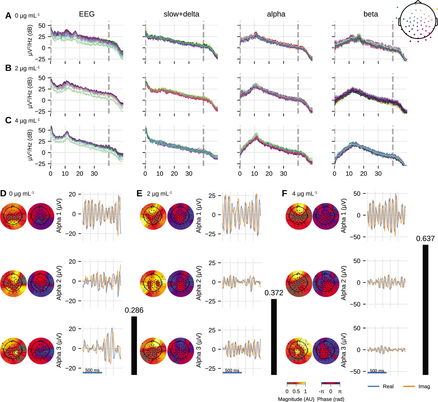
Oscillation component analysis (OCA) of the electroencephalogram (EEG) from a healthy volunteer undergoing propofol-induced unconsciousness.
Conditions of target effect-site concentration of (A, D) 0 (i.e., baseline), (B, E) , and (C, F) are analyzed. Panels (A–C) show the power spectral densities (PSDs) of reconstructed EEG activity within each canonical band. Panels (D–F) show the three dominant (in terms of sensor wide power) alpha component: the topographic maps show the magnitude (left) and phase (right) distribution of sensor-level mixing, the time courses are 1 s representative example of the extracted oscillations from the selected epochs. The black bars on the right display the coherency measure within alpha band. OCA correctly identifies that the spatial mixing sensor maps of the alpha waves (8–12 Hz) are oriented posteriorly at baseline, but gradually become frontally dominant under propofol. The sensor weights are scaled to have maximum value 1. So, the units of time series traces can be considered to be in µV.
Figure 5
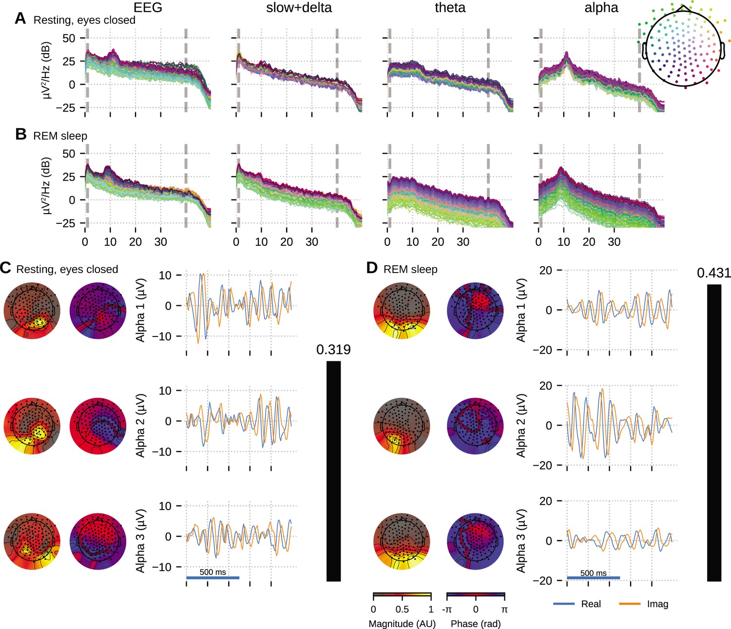
Oscillation component analysis (OCA) of the electroencephalogram (EEG) from a healthy young volunteer to compare between (A, C) wakeful resting state and (B, D) rapid eye movement (REM) sleep.
Panels (A, B) show the power spectral densities (PSDs) of reconstructed EEG activity within each canonical band. Panels (C, D) show the three dominant (in terms of sensor-wide power) alpha component: the topographic maps show the magnitude (left) and phase (right) distribution of sensor-level mixing, the time courses are 1 s representative example of the extracted oscillations from the selected epochs. The rightmost black bars display the coherency measure within alpha band. The contrasting topographic distribution of the alpha components (8–12 Hz), the shape of the oscillation power spectrum and alpha coherence hints at a distinct generating mechanism for alpha waves during stage 2 REM sleep compared to awake eyes closed alpha wave. The sensor weights are scaled to have a maximum value 1 so that the units of time series traces are in µV.
Figure 6
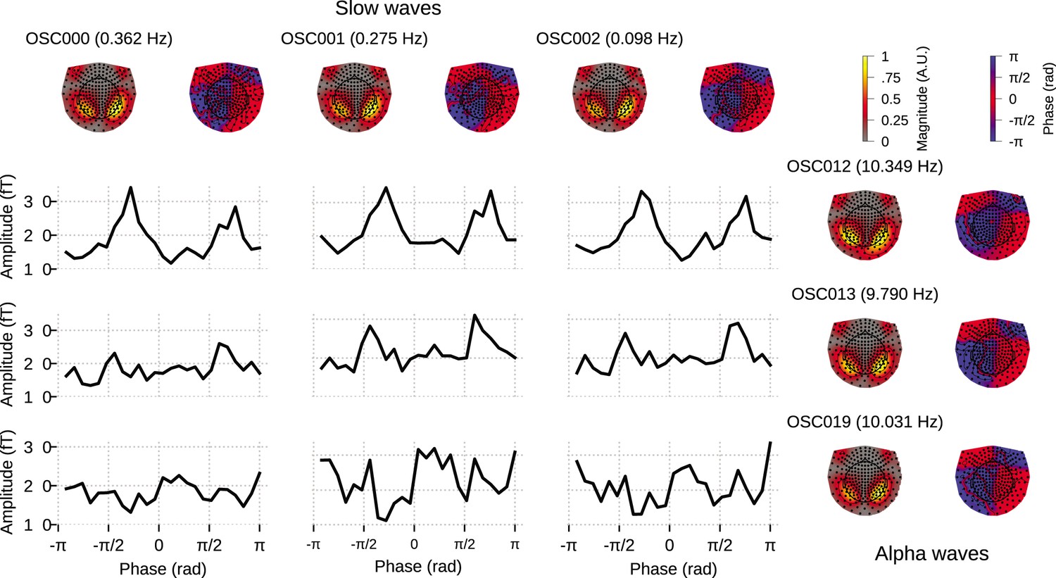
Cross–frequency phase–amplitude coupling in oscillation component analysis (OCA) components extracted from resting-state magnetoencephalogram (MEG) recording.
The black traces show the conditional mean of a selected alpha component (8–12 Hz) amplitude given another selected slow/delta component (0–4 Hz) phase. The three slow oscillations and three alpha oscillations that explained the highest variance were selected for demonstration purposes. The topographic maps show the magnitude (left) and phase (right) distribution of sensor-level mixing of the selected components.
Appendix 4—figure 1
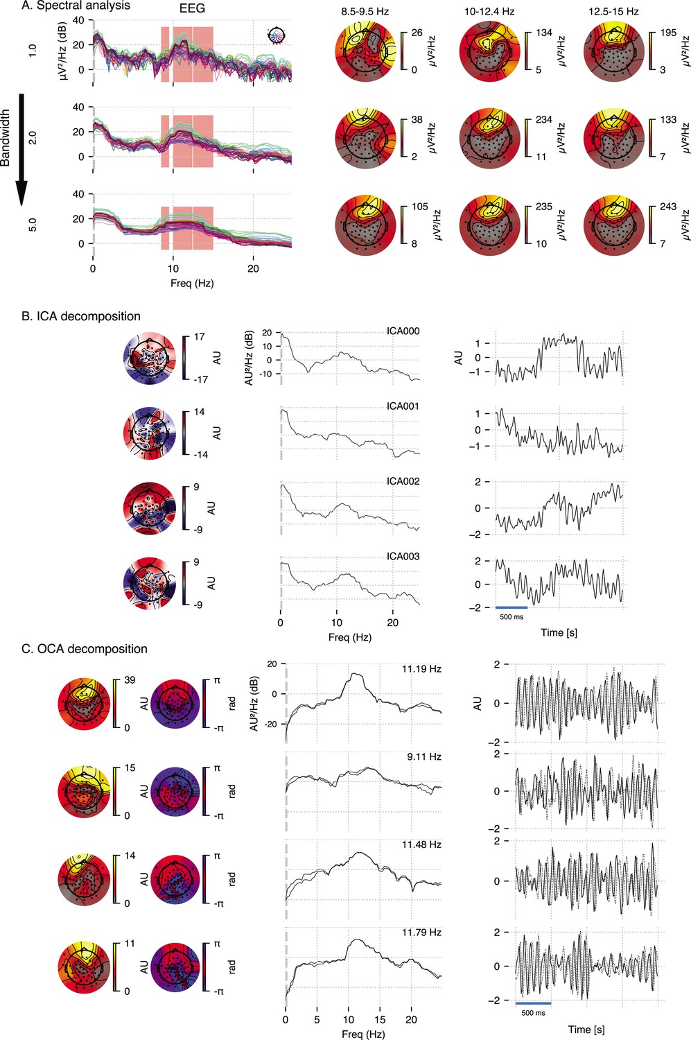
Empirical justification for oscillation component analysis (OCA) in analyzing real data.
A 3.5-s-long electroencephalogram (EEG) recording during propofol-induced anesthesia (effect-site concentration of 2 μg) is considered for this demonstration. (A) Power spectral density using multitaper method (for varying time-bandwidth product) of the EEG recording and power distribution over the EEG sensors in the marked frequency bands (red overlay) around visually identifiable peaks. (B) Four leading independent component analysis (ICA) components (left, middle, and right columns show topographic maps, power spectrum density, and time courses, respectively). (C) Four leading OCA components within alpha band (the topographic maps show the magnitude [left] and phase [right], while line plots show power spectrum density [left] and time-courses [right], respectively).
Tables
Key resources table
| Reagent type (species) or resource | Designation | Source or reference | Identifiers | Additional information |
|---|---|---|---|---|
| Software, algorithm | MNE-python 1.2 | https://mne.tools/stable/index.html; Gramfort et al., 2014 | ||
| Software, algorithm | Eelbrain 0.37 | https://eelbrain.readthedocs.io/en/stable/; Brodbeck et al., 2023 | ||
| Software, algorithm | purdonlabmeeg | This paper; Das, 2024 | Available at https://github.com/proloyd/purdonlabmeeg |
Additional files
Download links
A two-part list of links to download the article, or parts of the article, in various formats.
Downloads (link to download the article as PDF)
Open citations (links to open the citations from this article in various online reference manager services)
Cite this article (links to download the citations from this article in formats compatible with various reference manager tools)
A dynamic generative model can extract interpretable oscillatory components from multichannel neurophysiological recordings
eLife 13:RP97107.
https://doi.org/10.7554/eLife.97107.3


