An integrated machine learning approach delineates an entropic expansion mechanism for the binding of a small molecule to α-synuclein
- Tata Institute of Fundamental Research, India
Figures
Figure 1 with 12 supplements
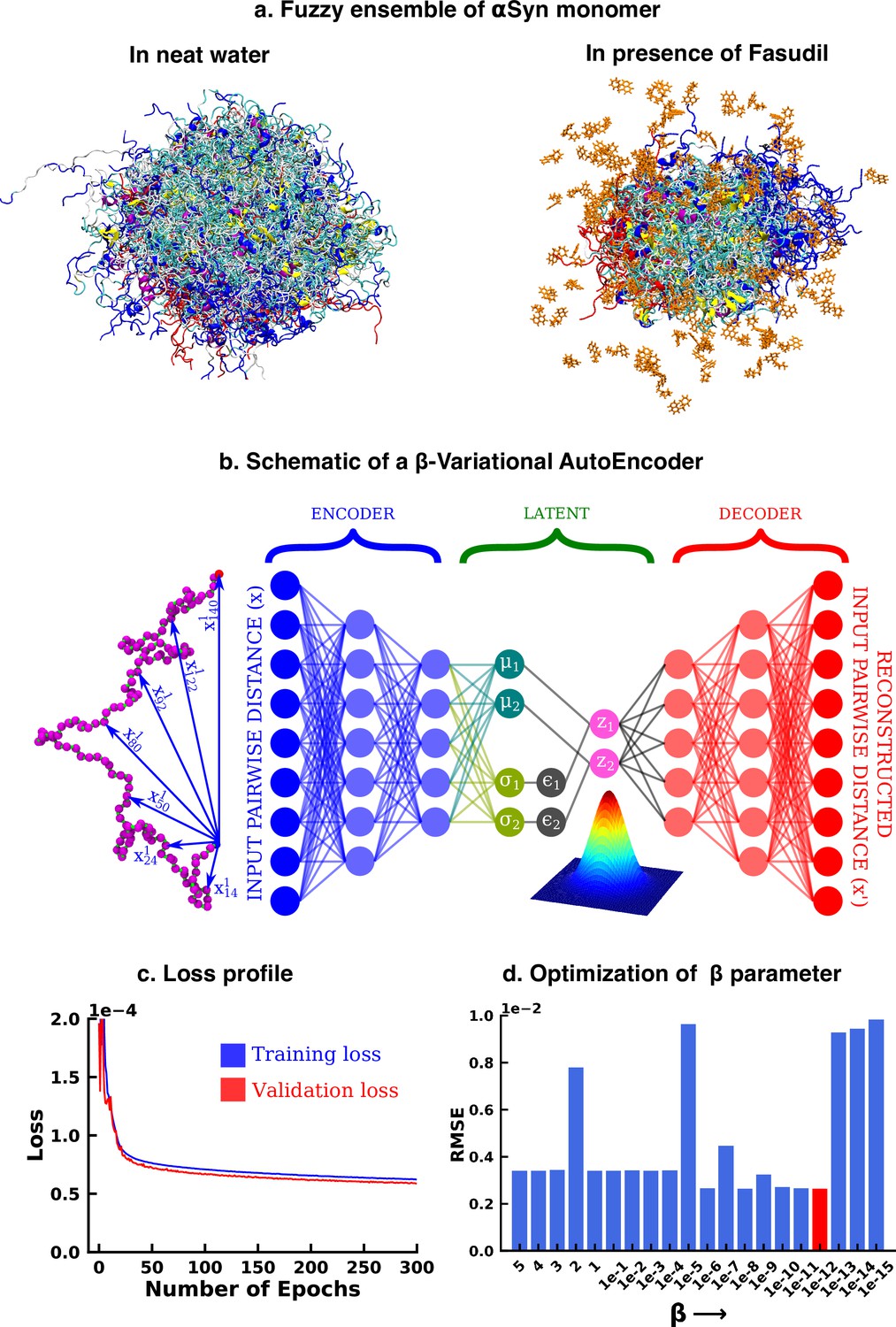
Deep neural network illustrating dimension reduction through β-Variational AutoEncoder.
(a) Conformational ensemble view of αS and αS-Fasudil ensemble, (b) A schematic of β-Variational Autoencoder (β-VAE), (c) Training and validation loss for β-VAE and (d) RMSE as a function of the β parameter. The red-annotated β parameter was used for the investigation.
Figure 1—figure supplement 1

Distribution of the radius of gyration (Rg) of the αS and αS-Fasudil ensembles.
The Rg values of the initial structures used for the αS and αS-Fasudil simulation sare marked as symbols. The red diamond is the Rg of the starting structure of the αS-Fasudil simulation and the blue triangle is the Rg of the starting structure of the αS simulations.
Figure 1—figure supplement 2

Distribution of end-to-end distance for the αS and αS-Fasudil ensembles.
The mean values of the distributions are marked.
Figure 1—figure supplement 3

Distribution of SASA for αS and αS-Fasudil ensembles.
The mean values of the distributions are marked.
Figure 1—figure supplement 4

Residue wise percentage secondary structure of helical nature in the αS and αS-Fasudil ensembles.
Figure 1—figure supplement 5
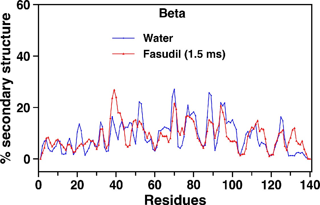
Residue wise percentage secondary structure of sheet nature in the αS and αS-Fasudil ensembles.
Figure 1—figure supplement 6

Residue wise percentage secondary structure of coil nature in the αS and αS-Fasudil ensembles.
Figure 1—figure supplement 7

Each blue diamond label represents the RMSD (nm) w.r.t the starting structure of aSyn-fasudil simulation.
The value associated with each diamond label corresponds to the timescale of simulation.
Figure 1—figure supplement 8

Fraction of helix content in the starting structures of the αS-Fasudil and αS simulations.
Figure 1—figure supplement 9

Fraction of β-sheet content in the starting structures of the αS-Fasudil and αS simulations.
Figure 1—figure supplement 10

Fraction of coil content in the starting structures of the αS-Fasudil and αS simulations.
Figure 1—figure supplement 11

Total SASA of the starting structures of the αS-Fasudil and αS simulations.
Figure 1—figure supplement 12

Residue wise SASA of the starting structure of the αS-Fasudil (red square) and αS (blue squares) simulations.
Figure 2
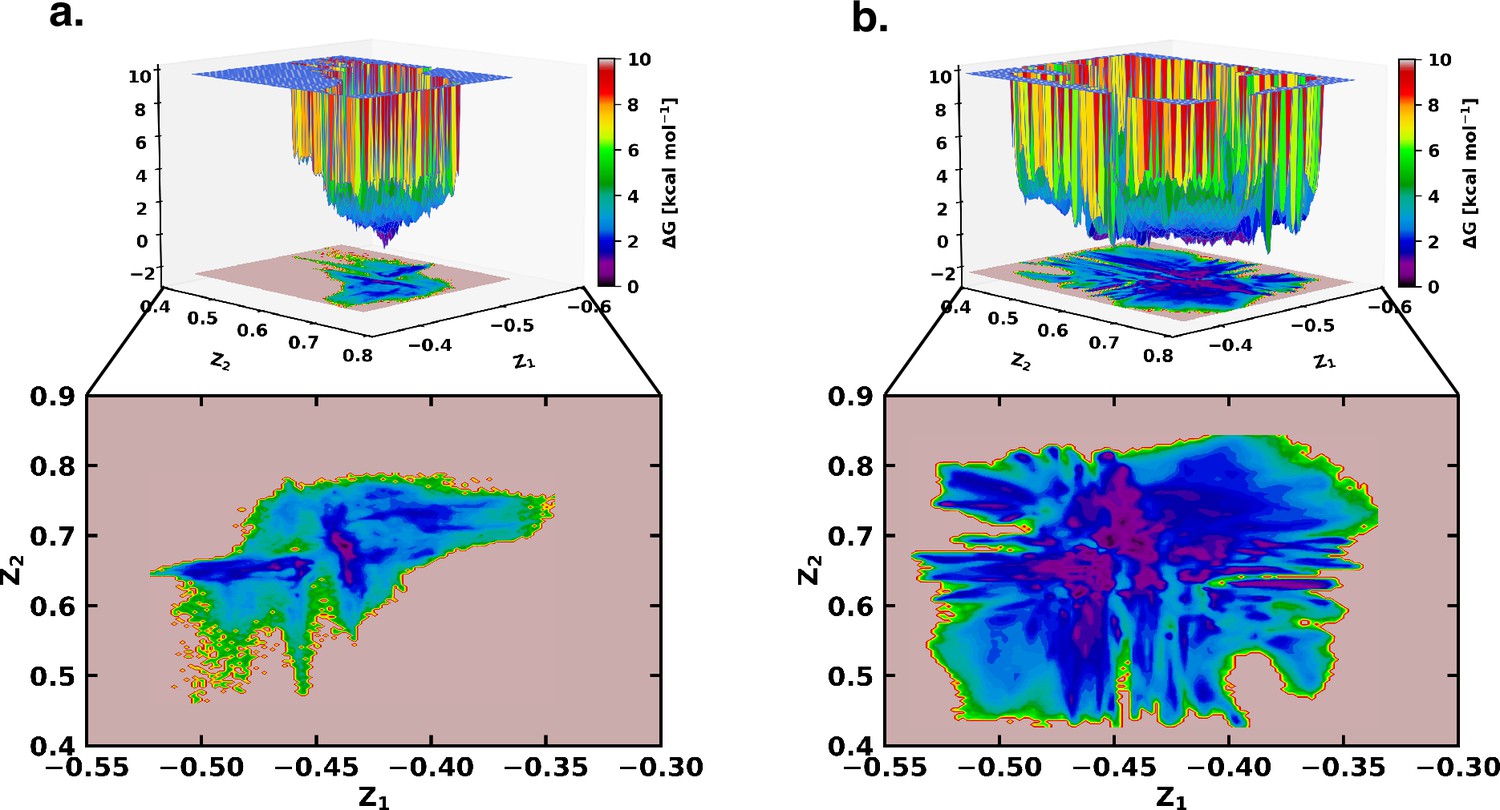
Free energy landscape using the latent space of β-VAE indicates greater conformational space sampled by αS in presence of fasudil.
The free energy landscape of (a) αS and (b) αS-Fasudil system as determined from the latent dimensions of β-VAE.
Figure 3 with 11 supplements
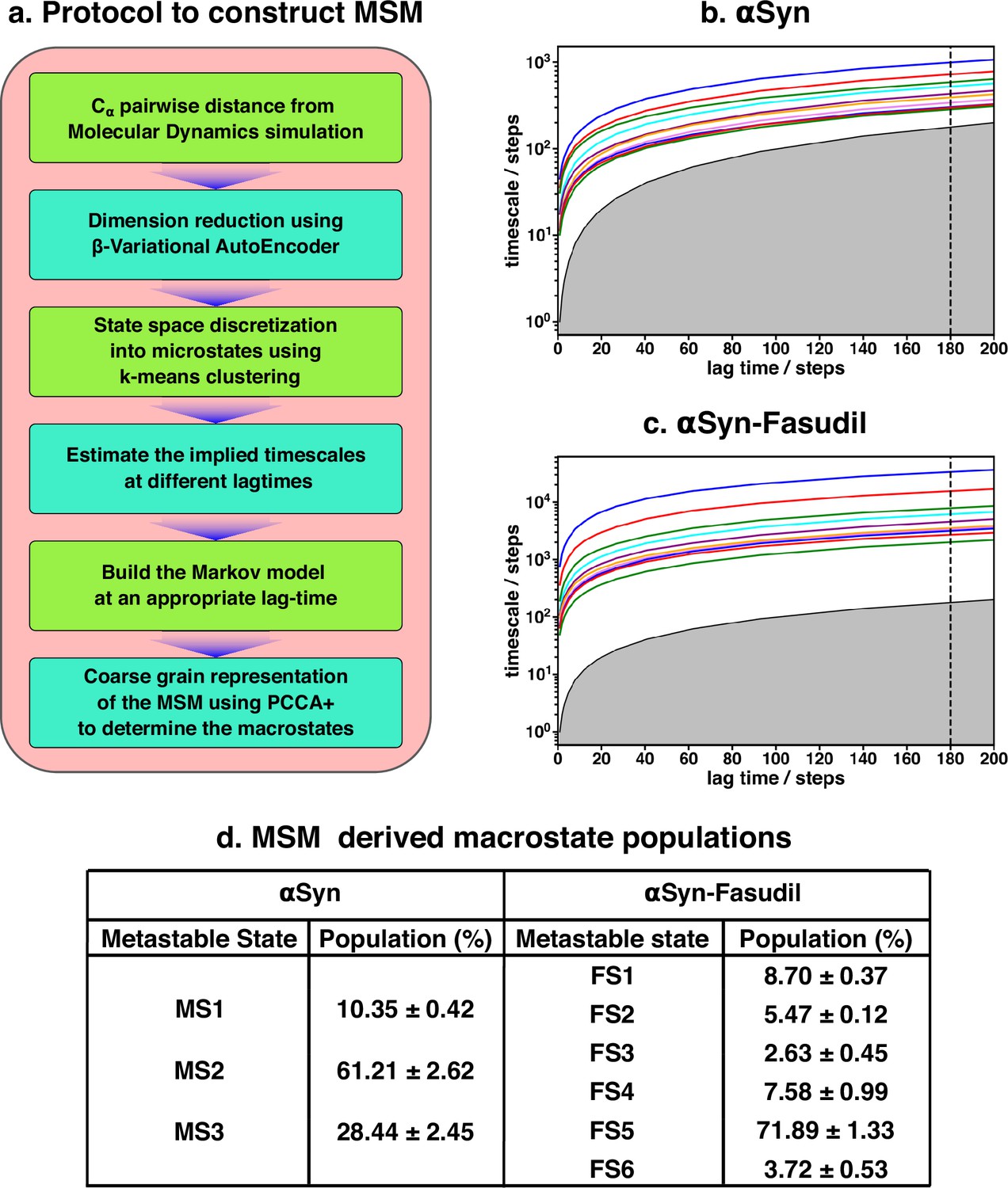
Markov state model captures three and six states of αS and αS-Fasudil system, respectively.
(a) A flowchart of the process of building a Markov State Model (MSM).(b, c) Implied timescales plot of the αS and αS-Fasudil systems. (c) Macrostate populations of the 3-state and 6-state MSM of the αS and αS-Fasudil systems. Bootstrapping was used to estimate the mean and standard deviations of the macrostate populations.
Figure 3—figure supplement 1
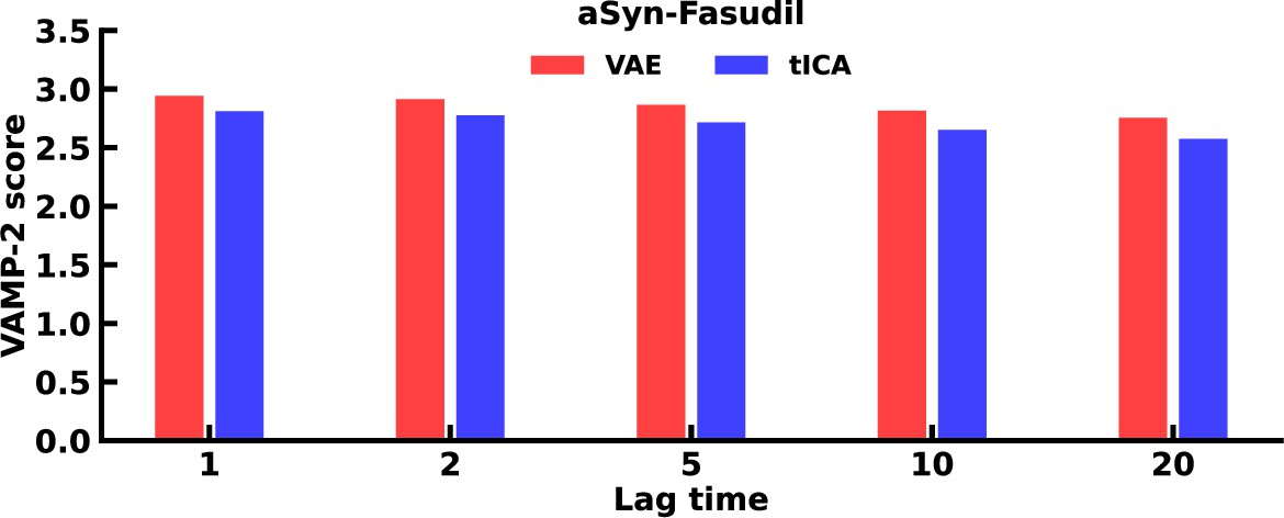
Comparison of VAMP-2 score from VAE and tICA of pairwise distances, reduced to two dimensions for the αS-Fasudil simulation.
Figure 3—figure supplement 2

Comparison of VAMP-2 score from VAE and tICA of pairwise distances, reduced to two dimensions for the αS simulation.
Figure 3—figure supplement 3
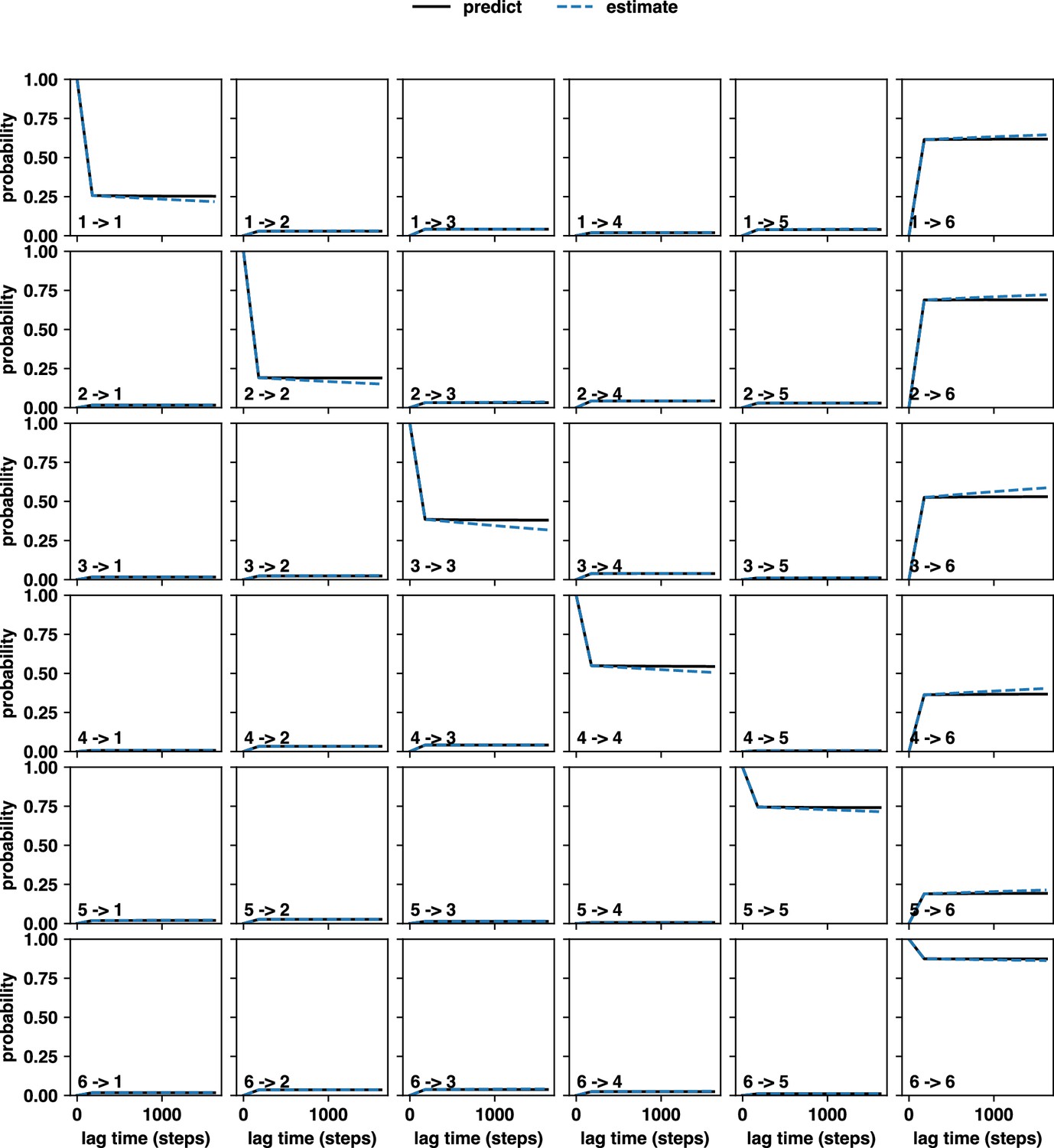
The Chapman-Kolmogorov test performed for the six state Markov State Model of the αS-Fasudil ensemble.
Figure 3—figure supplement 4

The implied timescale (ITS) plot αS-Fasudil simulation for the block of 10 μs to 70 μs.
Figure 3—figure supplement 5

Distribution of Rg of the αS ensemble and the 60 μs slice (10 μs-70 μs) of the αS-Fasudil simulation trajectory.
Figure 3—figure supplement 6

Distribution of Rg of the αS ensemble and the 60 μs slice (966 μs to 1026 μs) of the αS-Fasudil simulation trajectory.
Figure 3—figure supplement 7

The implied timescale (ITS) plot αS-Fasudil simulation for the block of 966 μs to 1026 μs.
Here too we see 6 states.
Figure 3—figure supplement 8

VAMP-2 score as a function of the number of microstates in for the αS-Fasudi ensembles for a latent space of four dimensions.
Figure 3—figure supplement 9

ITS plot of the αS-Fasudi simulation using the four dimension of the VAE.
Here too we see 6 states.
Figure 3—figure supplement 10

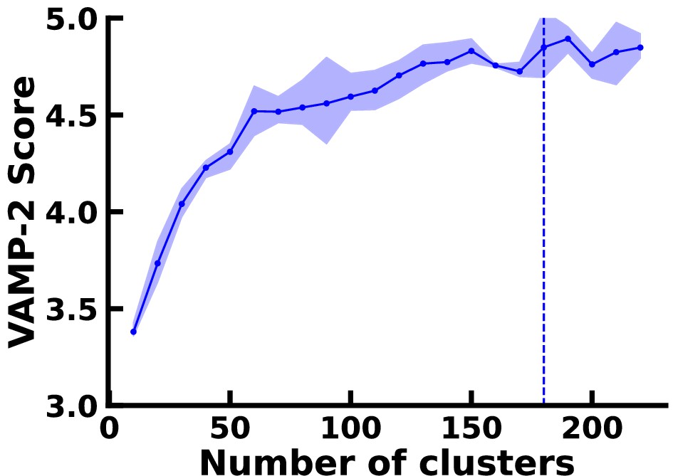
VAMP-2 score as a function of the number of microstates in for the αS-Fasudil ensemble.
Figure 3—figure supplement 11
VAMP-2 score as a function of the number of microstates in for the αS ensemble.
Figure 4 with 1 supplement
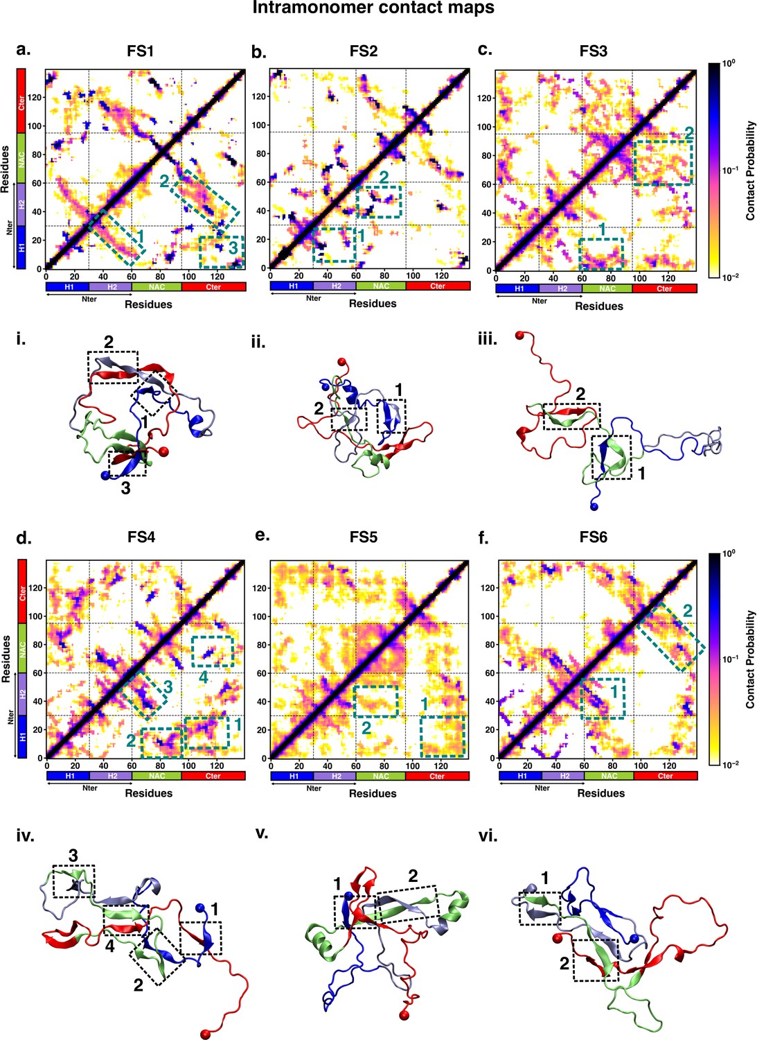
Intrapeptide residue-wise contact map of the macrostates of αS-Fasudil system indicates that the six states represent distinct ensembles.
Intrapeptide residue-wise contact probability maps of (a) six macrostates (FS1 to FS6) in the presence of fasudil. A contact is considered if the Cα atoms of two residues are within a distance of 8Å of eachother. Axes denote the residue numbers. The color scale for the contact probability is shown at the extreme right of each panel of maps. The color bar along the axes of the plots represents the segments in the αS monomer. Specific contact regions are marked by boxes and numbered. These contacts are illustrated by representative snapshots and the corresponding contacts are similarly marked and numbered.
Figure 4—figure supplement 1
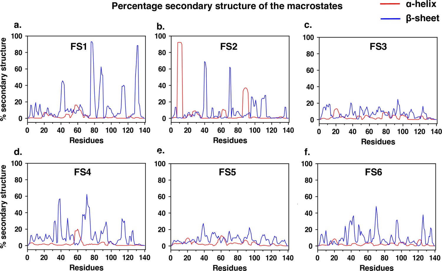
Residue-wise percentage secondary structure estimated for each of the six macrostates of αS monomer simulated in the presence of fasudil.
Figure 5 with 1 supplement
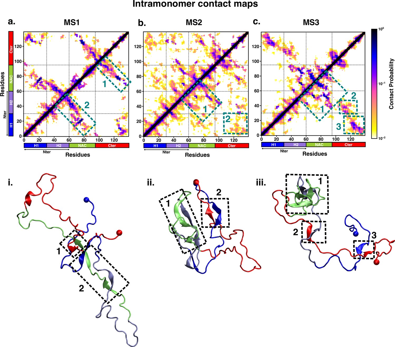
Intrapeptide residue-wise contact map of the macrostates of αS system indicates that the three states represent distinct ensembles.
Intrapeptide residue-wise contact probability maps of the three macrostates (MS1 to MS3) in neat water. A contact is considered if the Cα atoms of two residues are within a distance of 8Å of eachother. Axes denote the residue numbers. The color scale for the contact probability is shown at the extreme right. The color bar along the axes of the plots represents the segments in the αS monomer. Specific contact regions are marked by boxes and numbered. These contacts are illustrated by representative snapshots and the corresponding contacts are similarly marked and numbered.
Figure 5—figure supplement 1
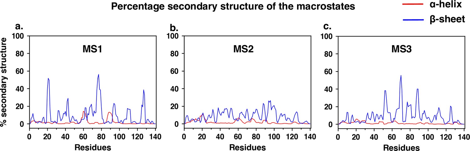
Residue-wise percentage secondary structure estimated for each of the three macrostates of αS monomer simulated in neat water.
Figure 6 with 4 supplements
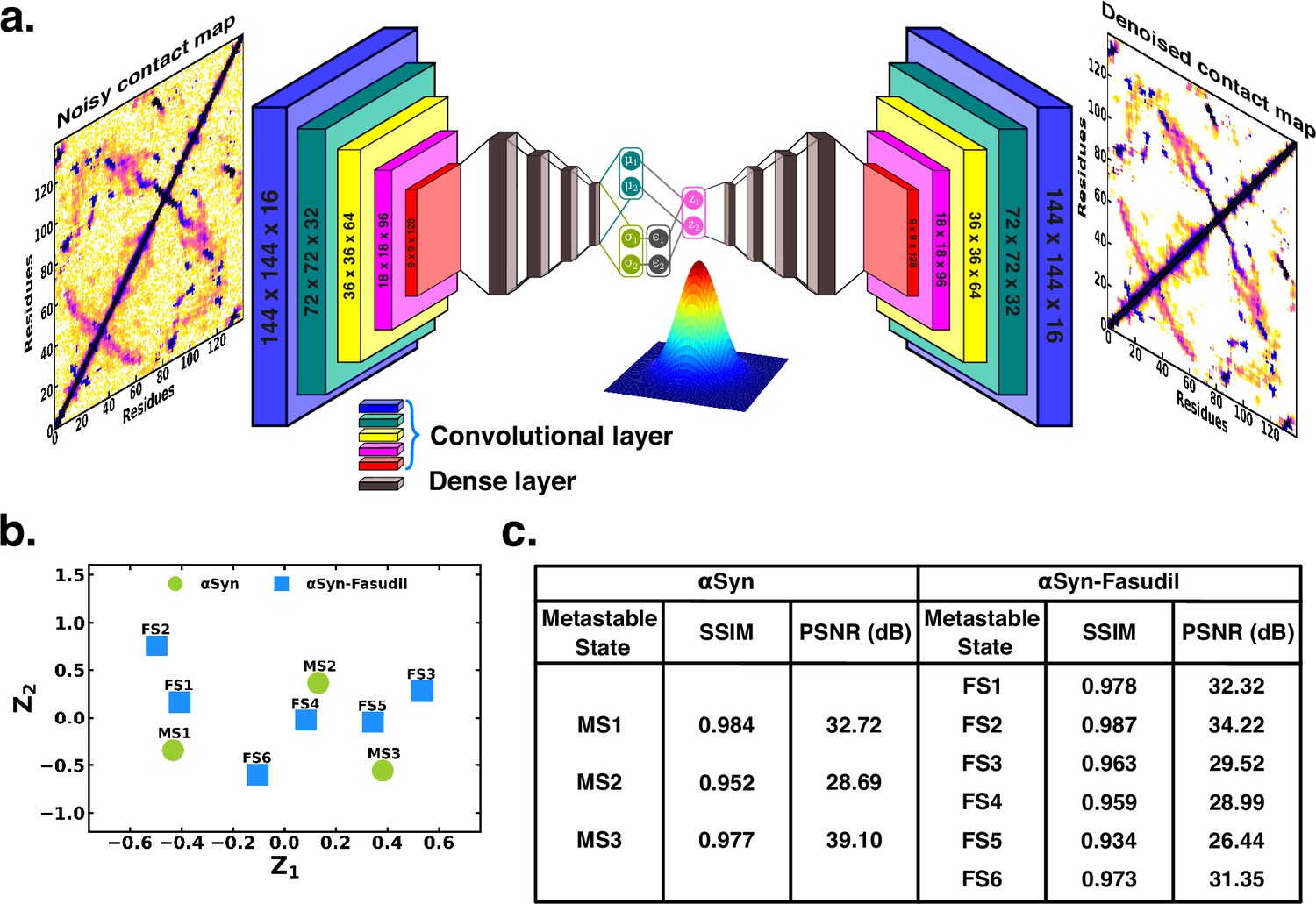
Projection of contact maps of αS and αS-Fasudil macrostates using denoising convolutional VAE.
(a) Schematic of denoising convolutional variational autoencoder (b) Latent space of the contact map of αS and αS-Fasudil metastable states. (c) SSIM and PSNR values for αS and αS-Fasudil metastable states.
Figure 6—figure supplement 1
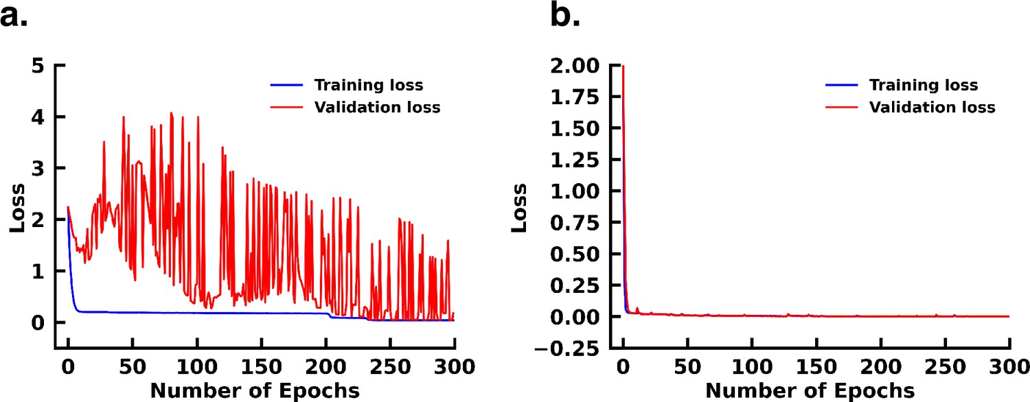
Loss profile of (a) CVAE indicating overfitting (b) DCVAE indicating no overfitting.
Figure 6—figure supplement 2
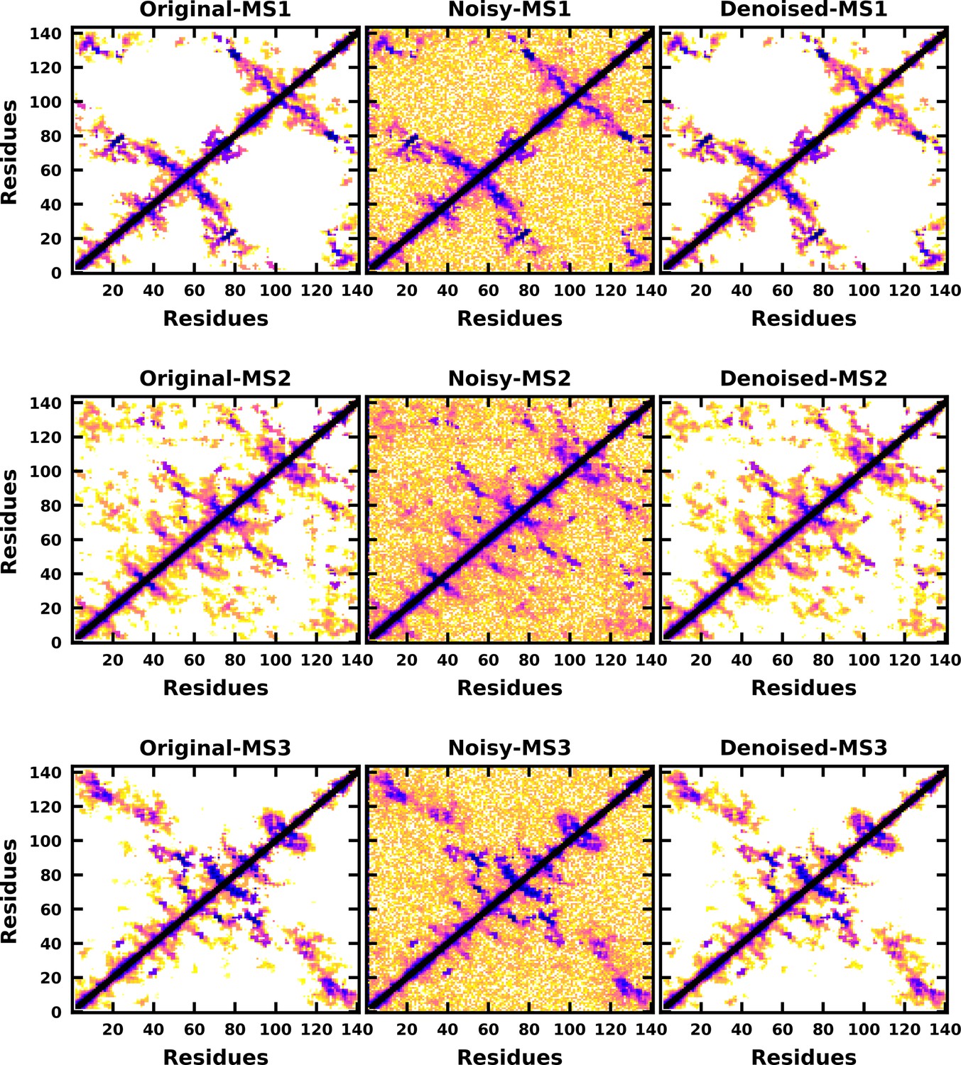
Denoised output of the contact map of the αS macrostates.
Figure 6—figure supplement 3
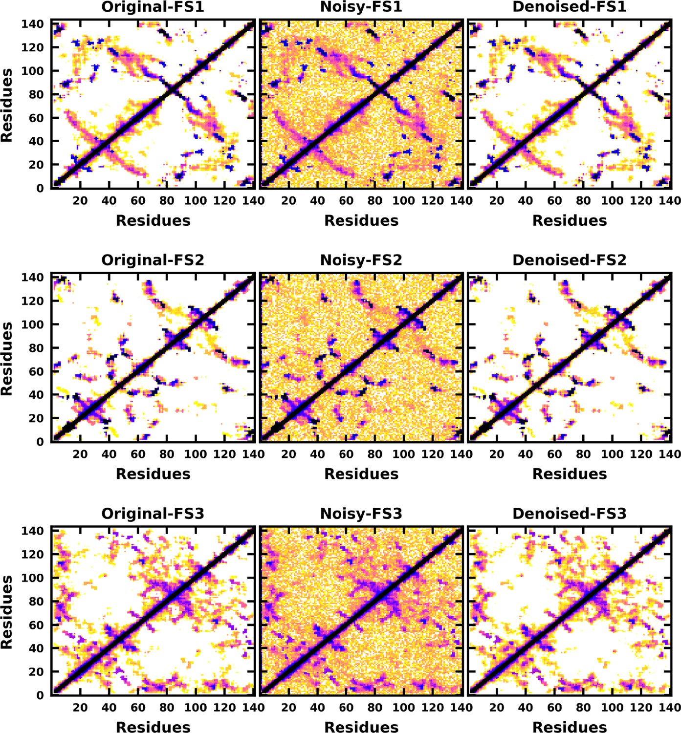
Denoised output of the contact map of the αS-Fasudil macrostates FS1, FS2, and FS3.
Figure 6—figure supplement 4
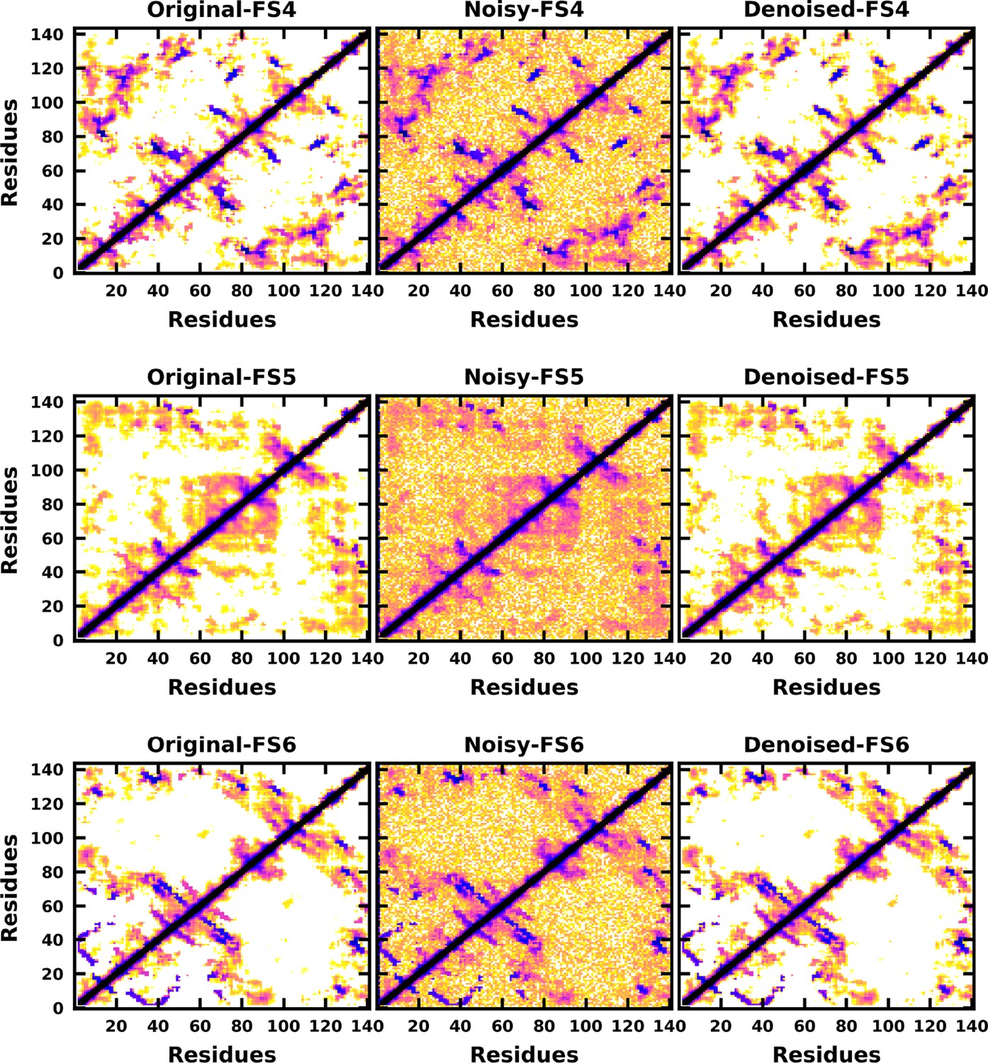
Denoised output of the contact map of the αS-Fasudil macrostates FS4, FS5, and FS6.
Figure 7
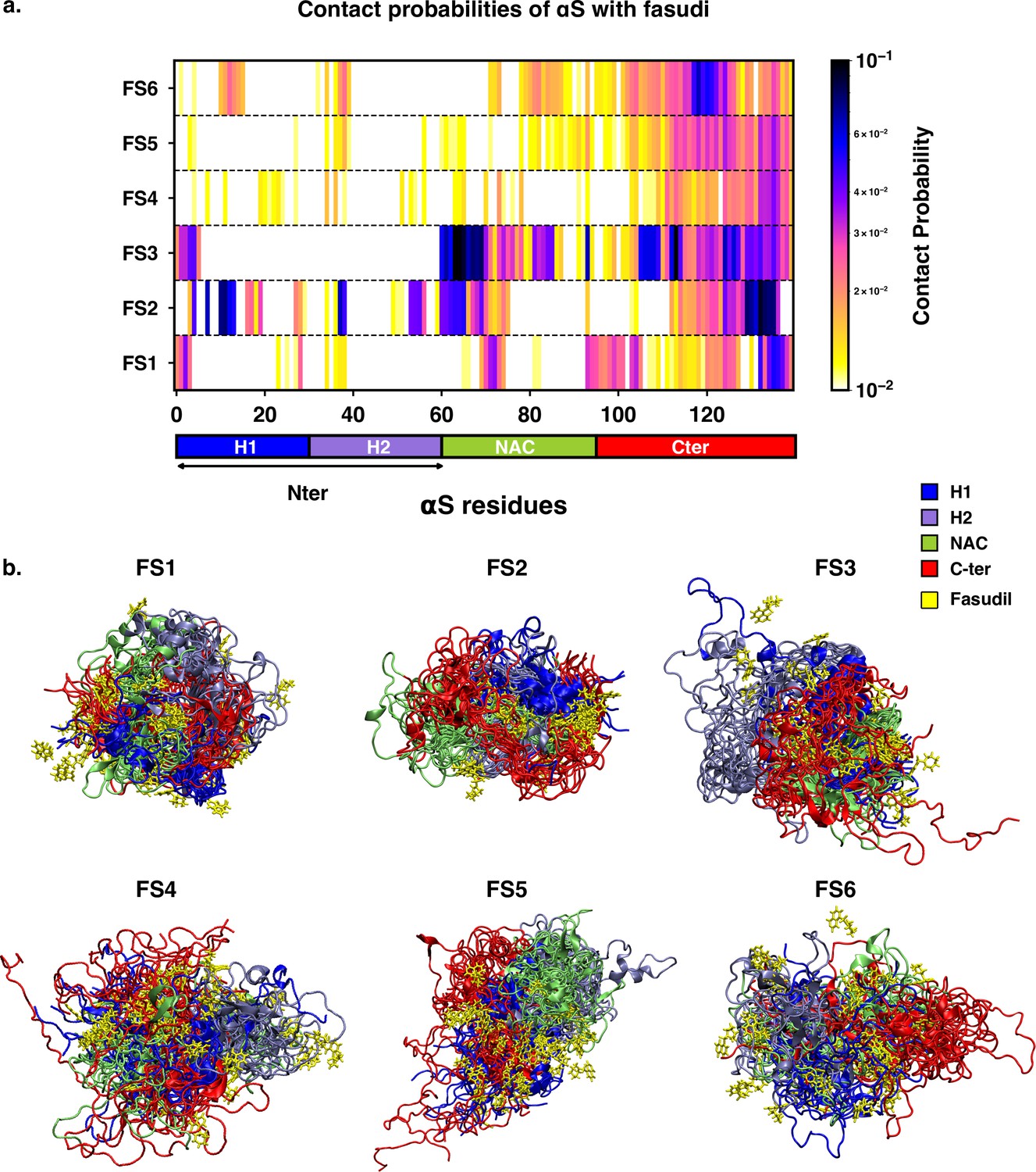
Contact map between fasudil and αS, indicates that fasudil interacts with distinct regions of αS in the six macrostates.
(a) Contact probability map of residue-wise interaction of fasudil with αS.(b) Overlay of representative conformations from the six macrostates (FS1 to FS6) along with the bound fasudil molecules. The conformations are colored segment-wise as shown in the legend. The fasudil molecules, in licorice representation, are colored yellow.
Figure 8 with 3 supplements
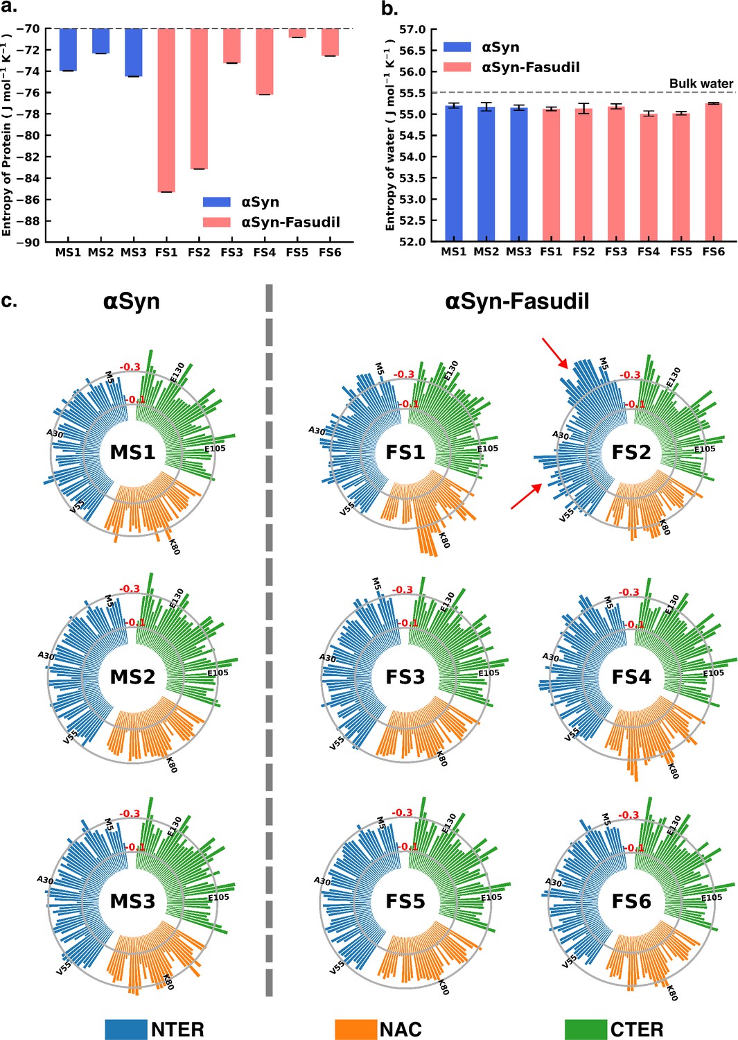
Entropy of αS system is modulated to a greater extent in presence of fasudil, with insignificant contribution from the solvent entropy.
(a) Total Protein entropy of the metastable states of αS and αS-Fasudil calculated from the torsion angles, relative to a fully flexible chain (b) Total water entropy in αS and αS-Fasudil system and (c) Residue-wise backbone entropy within the αS and αS-Fasudil states.
Figure 8—figure supplement 1
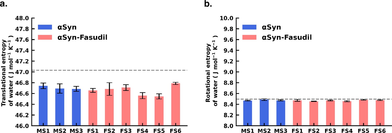
Translational and Rotational entropy of water.
(a) Translational entropy of water and (b) Rotational entropy of water in αS and αS-Fasudil system.
Figure 8—figure supplement 2
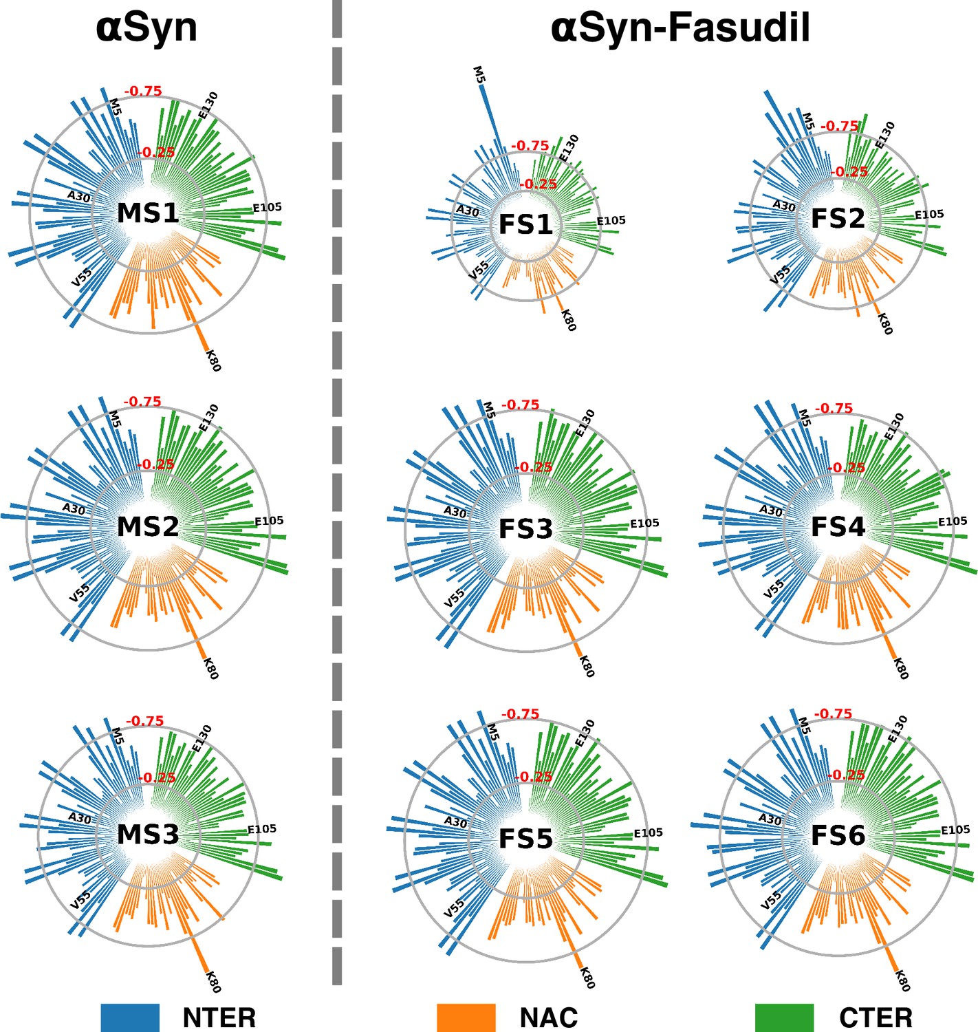
Residue-wise entropy of αS states populated in water and in the presence of fasudil.
Figure 8—figure supplement 3
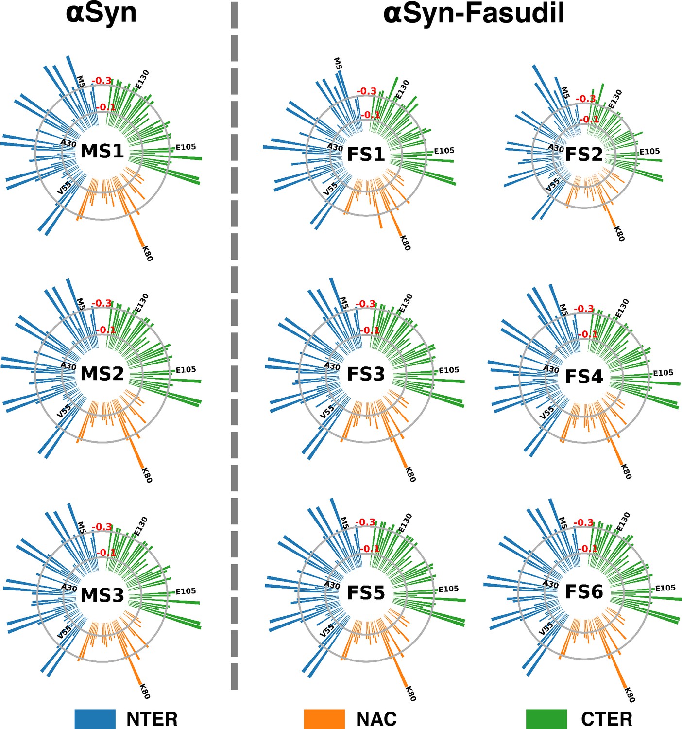
Residue-wise sidechain entropy of αS states populated in water and in the presence of fasudil.
Figure 9
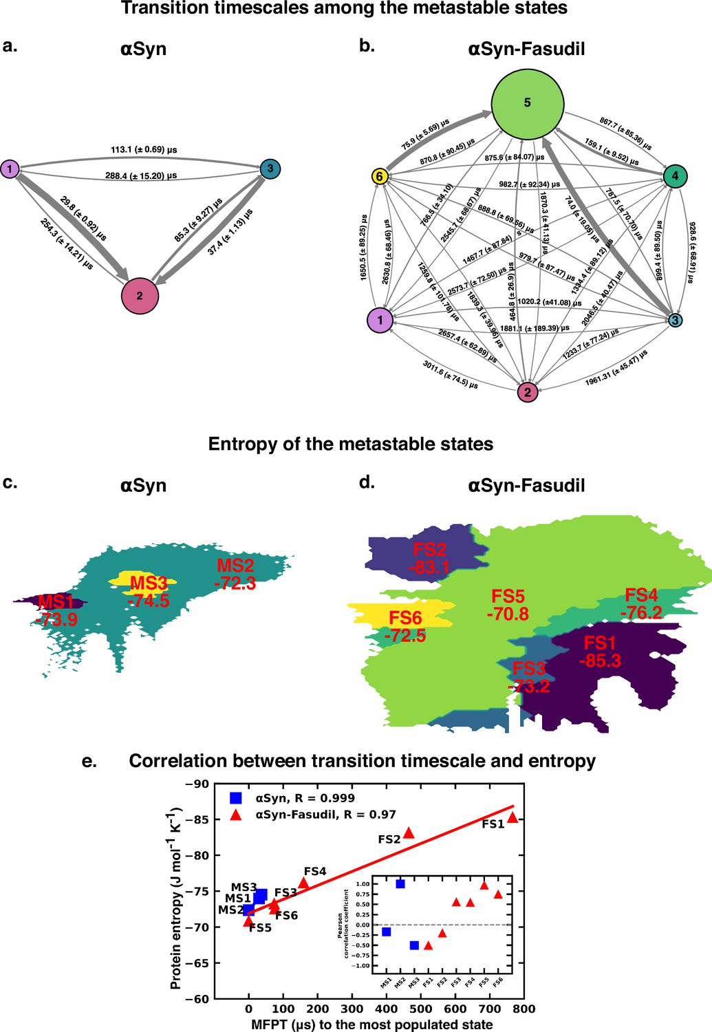
Mean first passage time for αS and αS-Fasudil ensembles indicates that a decrease in the transition time to the most entropic state in presence of fasudil, thereby potentially trapping S in the intermediate states.
The rate network obtained from MFPT analysis for the (a) 3-state MSM of the αS ensemble in neat water and (b) 6-state MSM of the αS-Fasudil ensemble. The sizes of the discs is proportional to the stationary population of the respective state. The thickness of the arrows connecting the states is proportional to the transition rate (1/MFPT) between the two states and the MFPT values are shown on the arrows. (c, d) Projection of conformation sub-ensemble PCCA +for αS and αS-Fasudil system in latent space, with respective protein entropy values (in unit of J mol-1 K -1) annotated on top of it. (e) Correlation between protein entropy and transition time to the major state for αS and αS-Fasudil system. The inset plot corresponds to the correlation between entropy and transition to the macrostate for αS and αS-Fasudl system.
Author response image 1

Left figure : Distribution of the radius of gyration (Rg) of the 23 apo simulation (as shown in the colourbar) and holo simulation (black).
Right figure : Mean and standard deviation (as error bar) of the Rg of the 23 apo (colourbar) and holo simulations (black).
Author response image 2

The Chapman-Kolmogorov test performed for the three state Markov State Model of the αS ensemble.
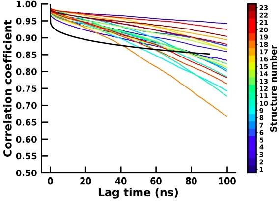
Author response image 3

Autocorrelation of the first principal component of the backbone dihedral for the apo (colourbar) and holo (black) simulation.
Author response image 4
Autocorrelation of the second principal component of the backbone dihedral for the apo (colourbar) and holo (black) simulation.
Author response image 5
Author response image 6

Distribution of (a)Rg, (b) Ree, (c) SASA and of the apo ensemble and a 60 μs slice of the holo simulation trajectory.
(d) ITS plot of the 60 μs chunk.
Author response image 7
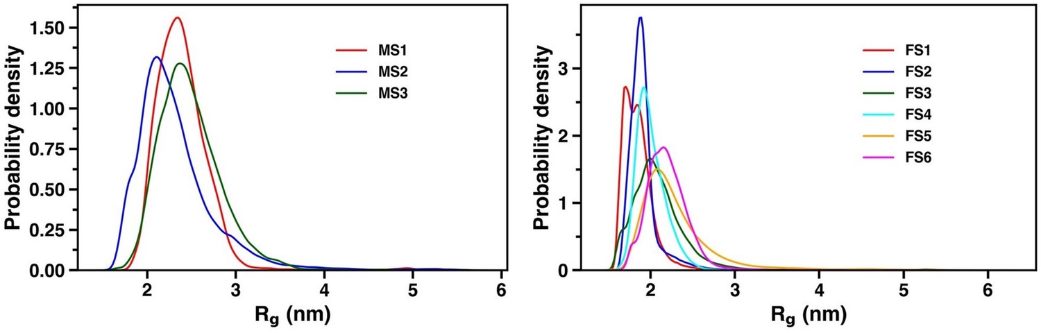
Distribution of radius of gyration for the three and six macrostates in the apo and holo simulation respectively.
Tables
Table 1
The size of the simulation box for the 23 αS simulations.
| Conformation number | Cubic Box size (nm) |
|---|---|
| 1 | 12.14 |
| 2 | 11.33 |
| 3 | 13.55 |
| 4 | 10.41 |
| 5 | 10.97 |
| 6 | 10.44 |
| 7 | 10.10 |
| 8 | 11.44 |
| 9 | 10.57 |
| 10 | 10.75 |
| 11 | 11.34 |
| 12 | 10.35 |
| 13 | 13.38 |
| 14 | 10.08 |
| 15 | 10.38 |
| 16 | 11.78 |
| 17 | 11.92 |
| 18 | 9.37 |
| 19 | 10.15 |
| 20 | 11.16 |
| 21 | 11.24 |
| 22 | 11.46 |
| 23 | 12.00 |
Additional files
Download links
A two-part list of links to download the article, or parts of the article, in various formats.
Downloads (link to download the article as PDF)
Open citations (links to open the citations from this article in various online reference manager services)
Cite this article (links to download the citations from this article in formats compatible with various reference manager tools)
An integrated machine learning approach delineates an entropic expansion mechanism for the binding of a small molecule to α-synuclein
eLife 13:RP97709.
https://doi.org/10.7554/eLife.97709.3


