Precision-based causal inference modulates audiovisual temporal recalibration
- Department of Psychology, New York University, United States
- Department of Psychology, University of Pennsylvania, United States
- Department of Psychology, Tufts University, United States
- Center for Neural Science, New York University, United States
Figures
Figure 1
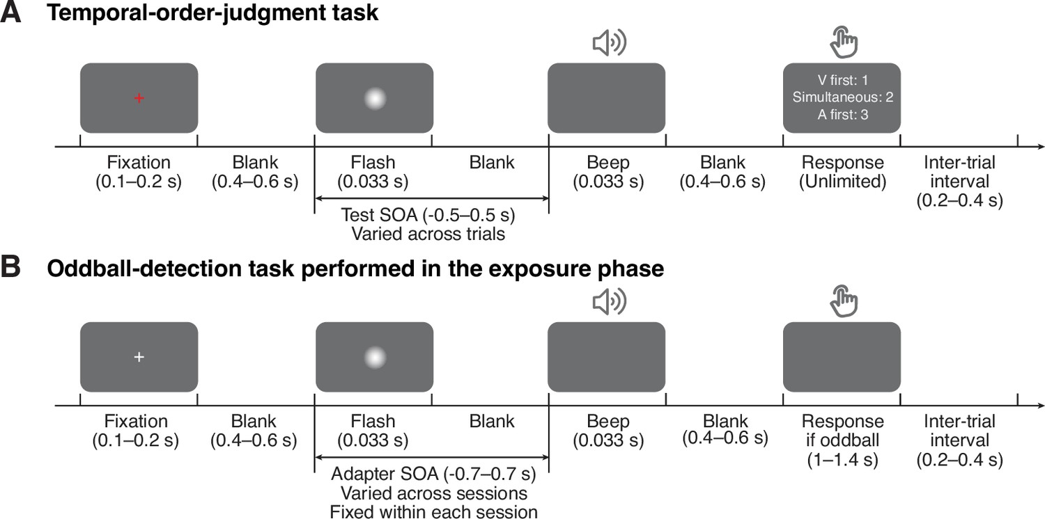
Task timing.
(A) Temporal-order judgment task administered in the pre- and post-tests. In each trial, participants made a temporal-order judgment in response to an audiovisual stimulus pair with a varying stimulus-onset asynchrony (SOA). Negative values: auditory lead; positive values: visual lead. The contrast of the visual stimulus was enhanced for illustration purposes. (B) Oddball-detection task performed in the exposure phase and top-up trials during the post-test phase. Participants were repeatedly presented with an audiovisual stimulus pair with an SOA that was fixed within each session but varied across sessions. Occasionally, the intensity of either one or both of the stimuli was increased. Participants were instructed to, whenever an oddball stimulus appeared, press a key indicating the modality of the oddball (visual, auditory, or both) .
Figure 2
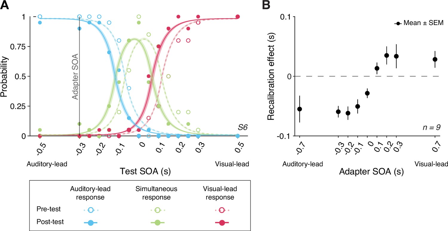
Behavioral results.
(A) The probability of reporting that the auditory stimulus came first (blue), the two arrived at the same time (green), or the visual stimulus came first (red) as a function of test stimulus-onset asynchrony (SOA) for a representative participant in a single session. The adapter SOA was –0.3 s for this session. Curves: best-fitting psychometric functions estimated jointly using the data from the pre-test (dashed) and post-test (solid). Shaded areas: 95% bootstrapped confidence intervals. (B) Mean recalibration effects averaged across all participants as a function of adapter SOA. The recalibration effects are defined as the shifts in the point of subjective simultaneity (PSS) from the pre- to the post-test, where the PSS is the physical SOA at which the probability of reporting simultaneity is maximized. Error bars: ± SEM.
Figure 3
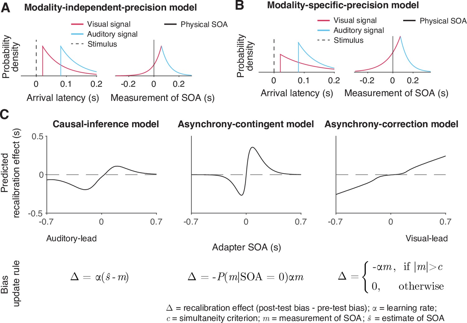
Illustration of the six observer models of cross-modal temporal recalibration.
(A) Left: Arrival-latency distributions for auditory (cyan) and visual (pink) sensory signals. When the precision of arrival latency is modality-independent, these two exponential distributions have identical shape. Right: The resulting symmetrical double-exponential measurement distribution of the stimulus-onset asynchrony (SOA) of the stimuli. (B) When the precision of the arrival latencies is modality-specific, the arrival-latency distributions for auditory and visual signals have different shapes, and the resulting measurement distribution of the SOA is asymmetrical. (C) Bias update rules and predicted recalibration effects for the three contrasted recalibration models: The causal-inference model updates the audiovisual bias based on the difference between the estimated and measured SOA. The asynchrony-contingent model updates the audiovisual bias by a proportion of the measured SOA and modulates the update rate by the likelihood that the measured sensory signals originated from a simultaneous audiovisual pair. The asynchrony-correction model adjusts the audiovisual bias by a proportion of the measured SOA when this measurement exceeds fixed criteria for simultaneity.
Figure 4
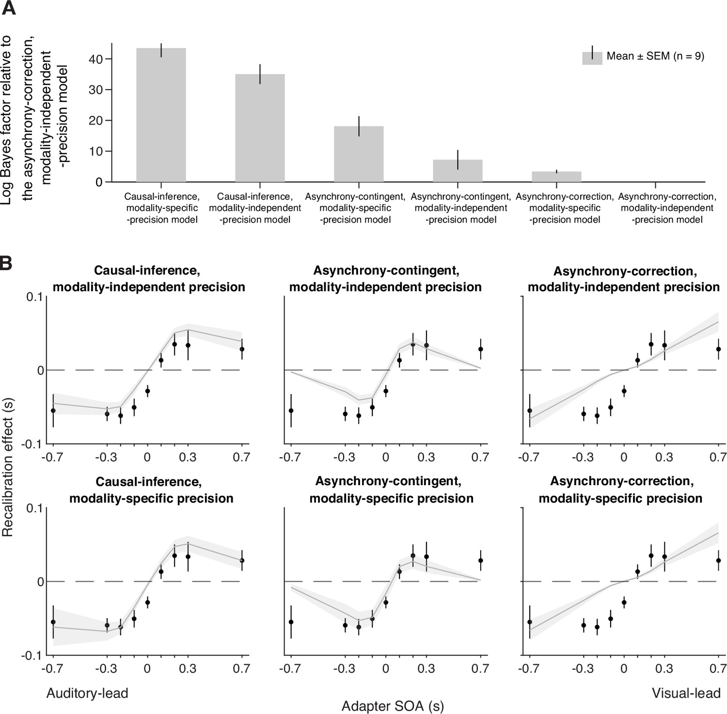
Model comparison and predictions.
(A) Model comparison based on model evidence. Each bar represents the group-averaged log Bayes factor of each model relative to the asynchrony-correction, modality-independent-precision model, which had the weakest model evidence. (B) Empirical data (points) and model predictions (lines and shaded regions) for the recalibration effect as a function of adapter stimulus-onset asynchrony (SOA).
Figure 5
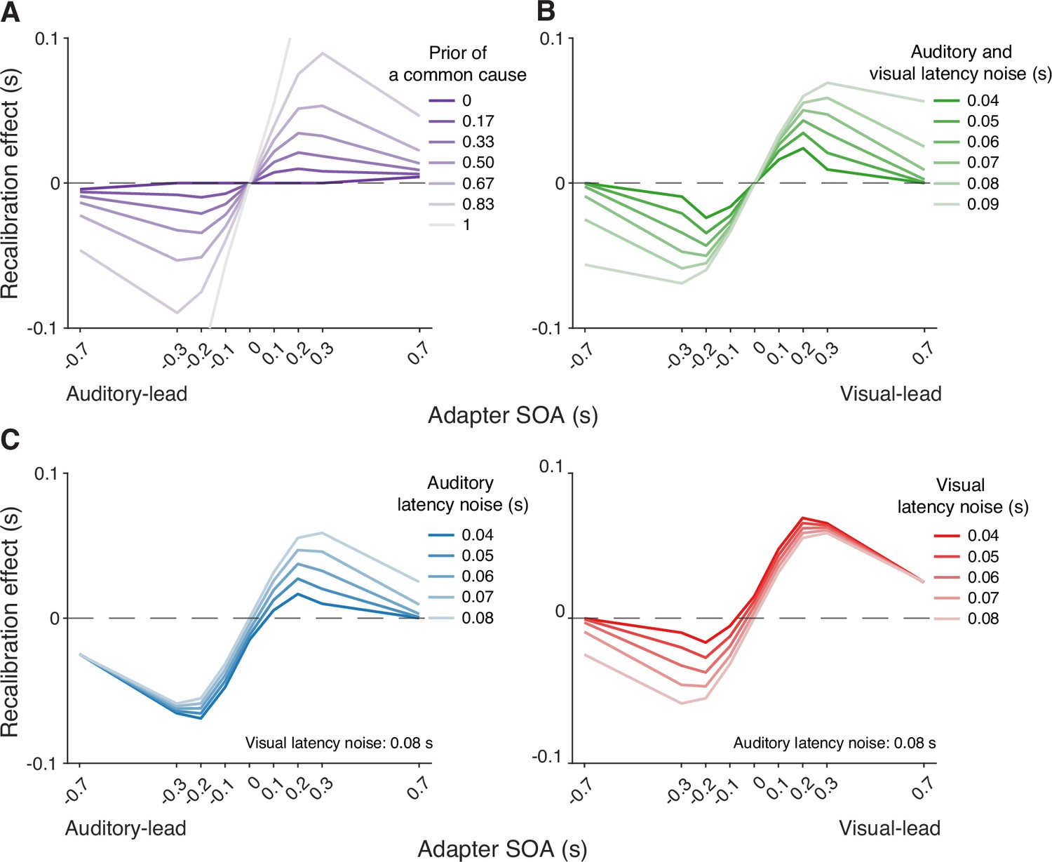
Simulation of temporal recalibration using the causal-inference model.
(A) The influence of the observer's prior belief of a common cause: the stronger the prior, the larger the recalibration effects. (B) The influence of latency noise: recalibration effects increase with decreasing sensory precision (i.e. increasing latency noise captured by the exponential time constant) of both modalities. (C) The influence of auditory/visual latency noise: recalibration effects are asymmetric between auditory-leading and visual-leading adapter stimulus-onset asynchronies (SOAs) due to differences in the precision of auditory and visual arrival latencies. Left panel: Increasing auditory latency precision (i.e. reducing auditory latency noise) reduces recalibration in response to visual-leading adapter SOAs. Right panel: Increasing visual precision (i.e. reducing visual latency noise) reduces recalibration in response to auditory-leading adapter SOAs.
Figure 6
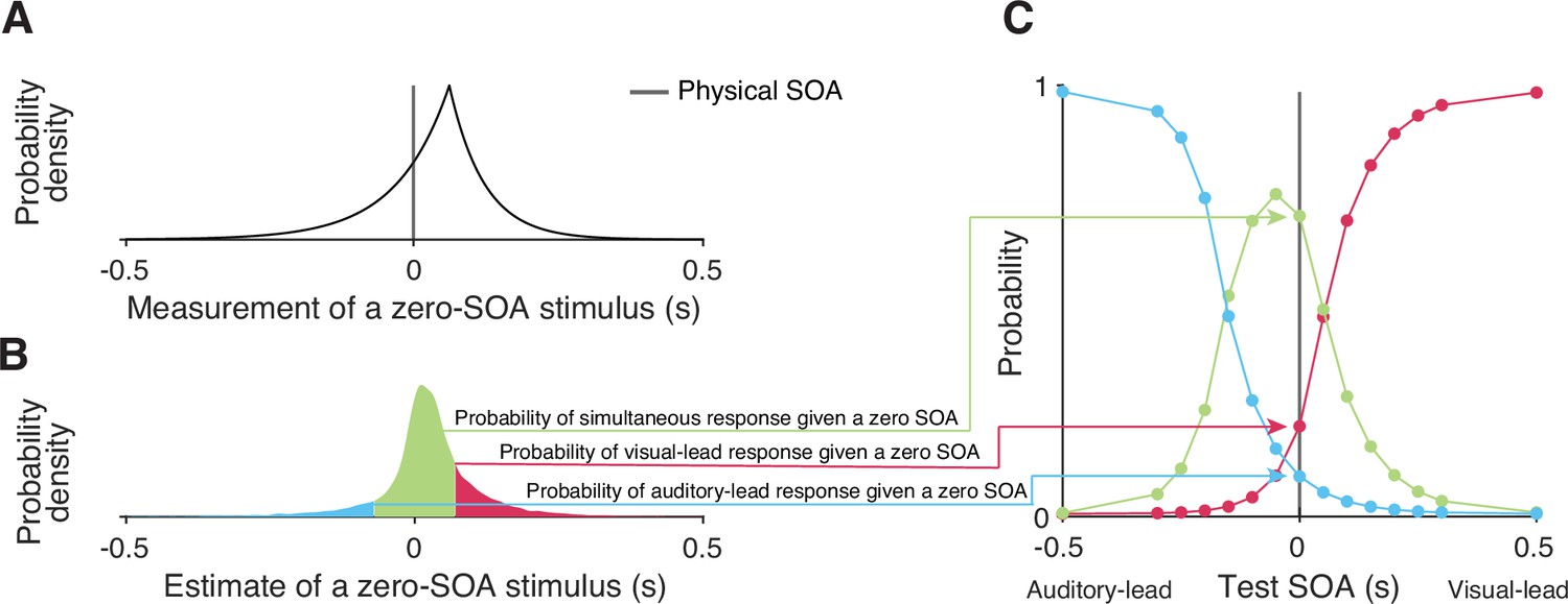
Simulating responses of the temporal-order-judgment (TOJ) task with a causal-inference perceptual process.
(A) An example probability density for the measurement of a zero stimulus-onset asynchrony (SOA). (B) The probability density of estimates resulting from a zero-SOA stimulus based on simulation using the causal-inference process. The symmetrical criteria around zero partition the distribution of estimated SOA into three regions, coded by different colors. The area under each segment of the estimate distribution corresponds to the probabilities of the three possible intended responses for a zero SOA. (C) The simulated psychometric function computed by repeatedly calculating the probabilities of the three response types across all test SOAs.
Appendix 1—figure 1
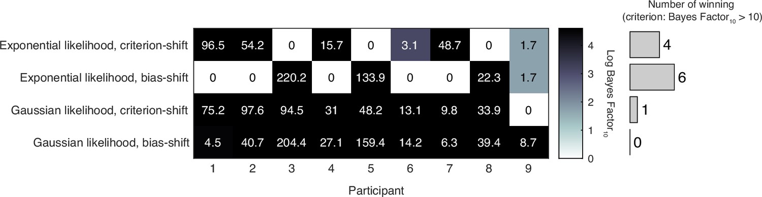
Model comparison results of the atheoretical models.
The model with the largest log model evidence is determined to be the best-fitting model for each participant. The table displays the log Bayes factor of each model relative to the best-fitting model for each participant. Thus, the best-fitting model has a relative log Bayes factor of zero. Larger values for other models indicate stronger support for the best-fitting model. The vertical histogram shows the number of participants for which each model was the best fit, based on the criterion that a model is rejected if its relative log Bayes factor is greater than log(10) = 2.3.
Appendix 2—figure 1
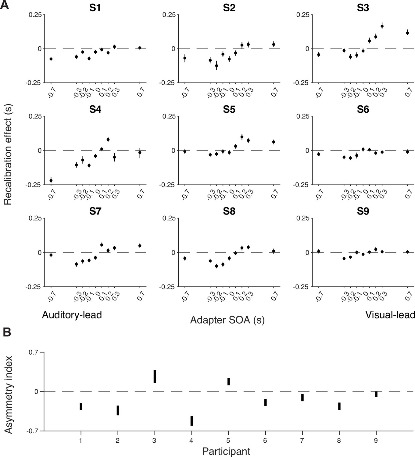
Individual-level recalibration effect.
(A) Individual recalibration effect estimated from the atheoretical model that assumes a bias shift and double-exponential measurement distribution. Error bars: 95% confidence interval of recalibration amount from 1000 bootstrapped datasets for that participant. (B) The 95% confidence interval of the asymmetry index (i.e. summed recalibration amount across adapter SOAs) from 1000 bootstrapped datasets for each participant. The confidence interval for all except the last participant excluded zero (CI of S9: [–0.093, 0.006]), suggesting a general asymmetry in recalibration.
Appendix 4—figure 1

Model comparison results of the recalibration models.
The table displays log Bayes factor relative to the best-fitting model for each participant. Thus, the best-fitting model has a relative log Bayes factor of 0. Larger values for other models indicate stronger support for the best-fitting model. The vertical histogram shows the number of participants for which each model was the best fit, based on the criterion that a model is rejected if the log Bayes factor relative to the best-fitting model is greater than log(10) = 2.3.
Appendix 5—figure 1
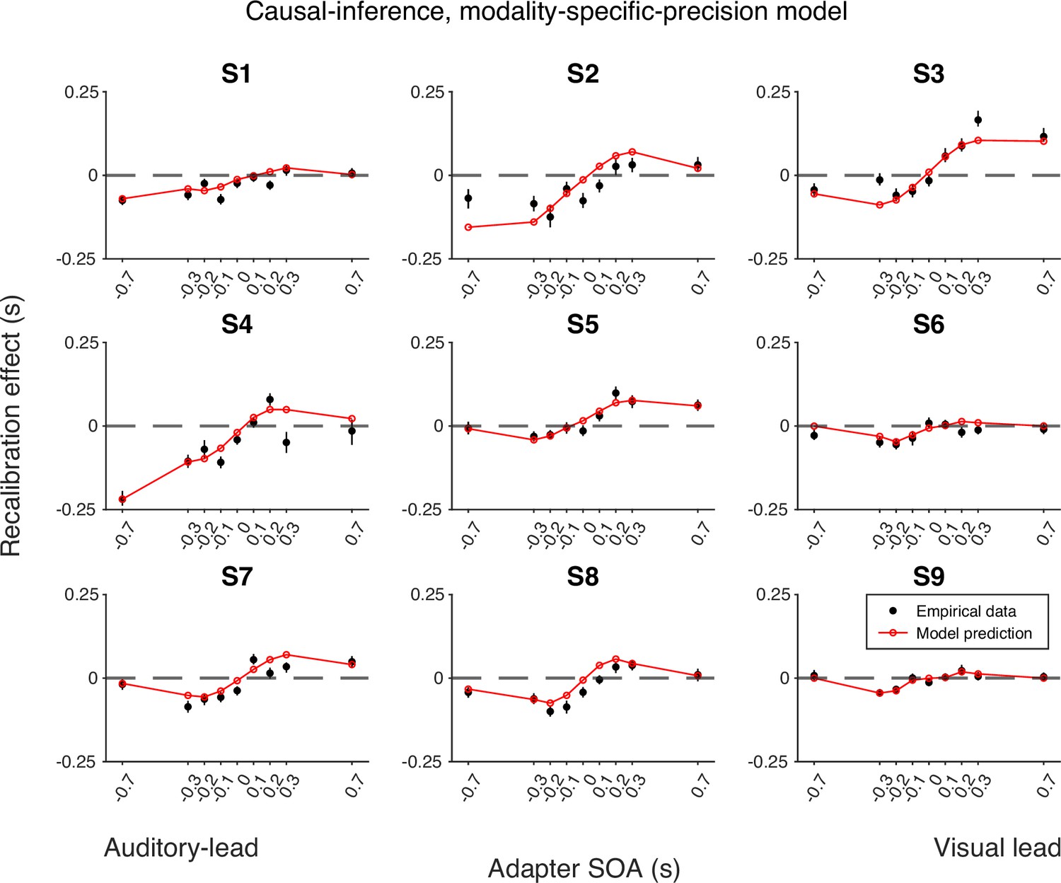
Empirical data for the recalibration effect for each participant and model predictions of the causal-inference recalibration model with modality-specific precision.
Each panel represents a single participant. Black dots: empirical estimates from the best atheoretical model (the bias-shift model with exponential likelihood). Error bars: the 95% bootstrapped confidence intervals. Red lines: predictions of the recalibration model from the best-fitting parameter estimates for that participant.
Appendix 5—figure 2
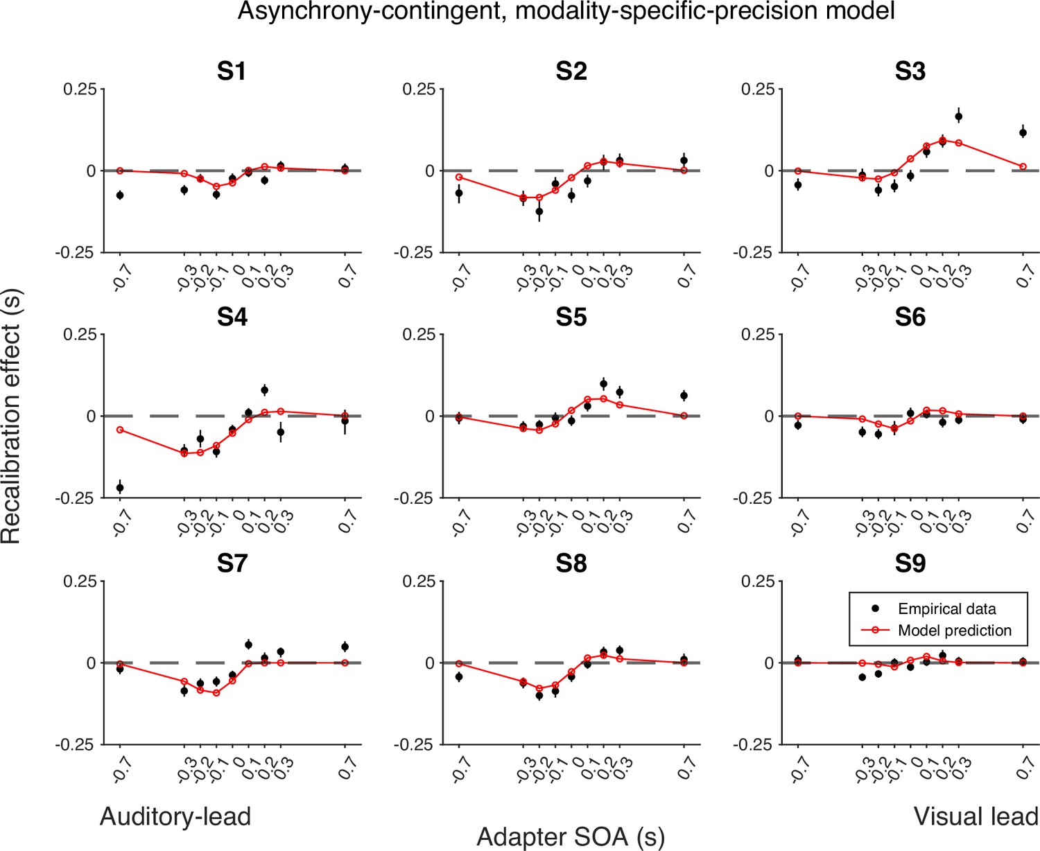
Empirical data of the recalibration effect for each participant and model predictions of the asynchrony-contingent recalibration model with modality-specific precision.
Each panel represents a single participant. Black dots: empirical estimates from the best atheoretical model (the bias-shift model with exponential likelihood). Error bars: the 95% bootstrapped confidence intervals. Red lines: predictions of the recalibration model from the best-fitting parameter estimates for that participant.
Appendix 5—figure 3
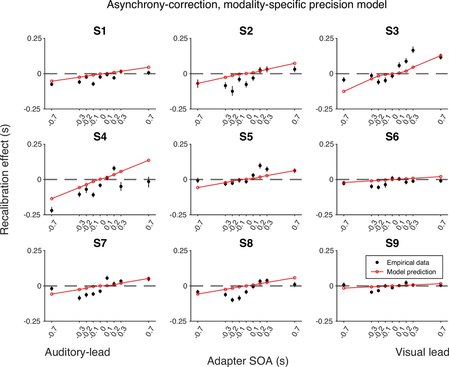
Empirical data of the recalibration effect for each participant and model predictions of the asynchrony-correction recalibration model with modality-specific precision.
Each panel represents a single participant. Black dots: empirical estimates from the best atheoretical model (the bias-shift model with exponential likelihood). Error bars: the 95% bootstrapped confidence intervals. Red lines: predictions of the recalibration model from the best-fitting parameter estimates for that participant.
Appendix 6—figure 1
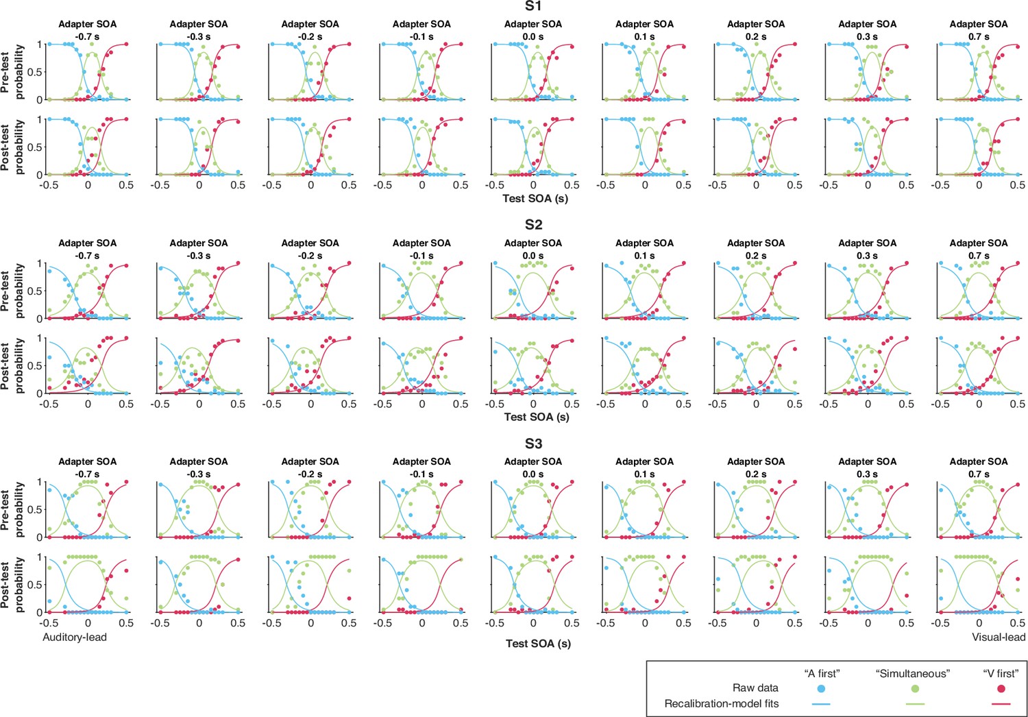
Data and predictions of the causal-inference, modality-specific-precision model for the temporal-order-judgment responses for each participant (S1–S3).
Appendix 6—figure 2
Data and predictions of the causal-inference, modality-specific-precision model for the temporal-order-judgment responses for each participant (S4–S6).
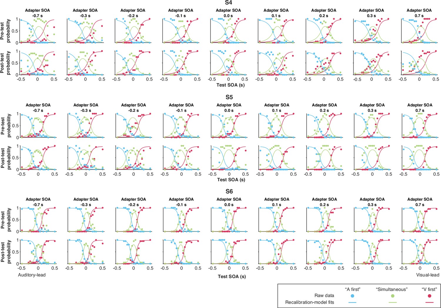
Appendix 6—figure 3
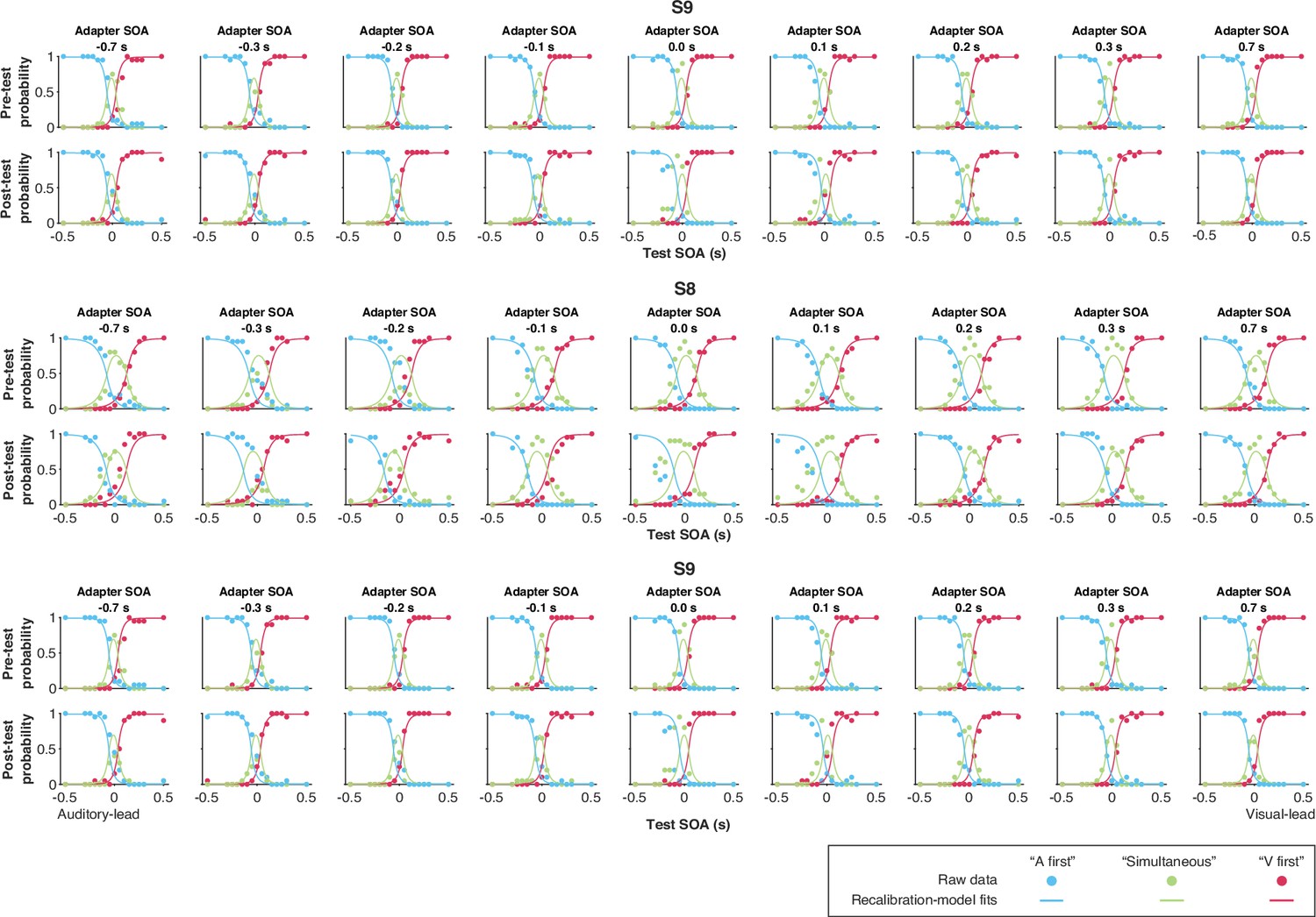
Data and predictions of the causal-inference, modality-specific-precision model for the temporal-order-judgment responses for each participant (S7–S9).
Appendix 7—figure 1
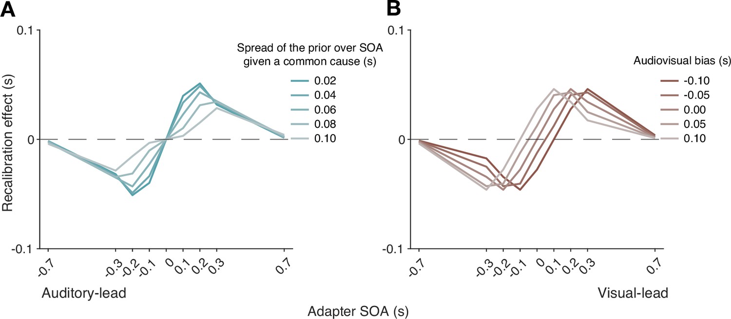
The effect of the spread of the prior over SOA given a common cause on recalibration.
(A) A smaller spread increases the recalibration magnitude, but only for a small SOA range where the probability of a common cause is higher. (B) The effect of the audiovisual temporal bias on recalibration. Audiovisual temporal bias affects where recalibration starts in the direction of the other modality, but its effects are reduced for large adapter SOAs. Overall, temporal bias shifts the recalibration function laterally, with minimal impact on the asymmetry of recalibration effect.
Appendix 8—figure 1

Simulation of a population-code model with varying adapter SOA.
(A) Left panel: Tuning curves of a neural population adapted to a 175 ms SOA, with 29 neurons having preferred SOAs that range from –500 to 500 ms. Middle panel: Neural responses to a stimulus with 0 ms SOA before (solid) and after (dashed) adaptation to a 175 ms SOA. Green: physical 0 ms SOA. Purple: estimated SOA based on an adaptation-unaware maximum-likelihood readout of the population response after adaptation. Right panel: Bias (i.e. estimated SOA minus physical SOA) across different stimulus SOAs after adaptation to a 175 ms SOA. (B) The same as in (A) after adaptation to a 525 ms SOA. (C) Bias as a function of stimulus SOA for several adapter SOAs. (D) Recalibration effect (i.e. the points of subjective simultaneity [PSS]: the stimulus SOA leading to an estimate of a 0 ms SOA) assuming an unbiased PSS before adaptation.
Appendix 9—figure 1

Temporal-order judgments from the outlier participant.
We excluded this participant's data because the probabilities of the three responses were similar across test stimulus-onset asynchronies (SOAs). These responses were too noisy to constrain the psychometric function.
Appendix 10—figure 1

Oddball-detection performance in the exposure and post-test phases.
Each dot represents a participant. In each phase, we combined responses across sessions and computed hit rates and false-alarm rates for auditory and visual oddballs. For each modality, hit and false-alarm rates were the probability of reporting an oddball when an oddball was presented and when it was absent, respectively. The resulting values for each participant confirm that they engaged in the task and attended to both modalities during the exposure phase. In general, participants showed a higher for auditory oddballs compared to visual ones, despite our attempt to equate performance levels. Furthermore, the remained consistent from the exposure to post-test phases, indicating similar performance in the top-up trials to performance during the exposure phase.
Appendix 11—figure 1
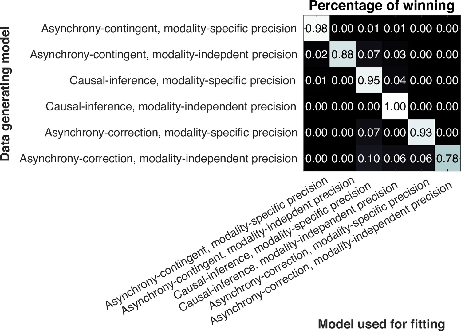
Confusion matrix resulting from the model-recovery simulations.
Each cell indicates the proportion of the 100 simulations for each model generating the data that were best fit by each of the six models (i.e. the values in each row sum to one).
Appendix 12—figure 1

Confusion matrix resulting from the model-recovery simulations.
Update model: the alternative model assuming that causal inference modulates recalibration at the bias-update phase. Percept model: the model described in the main text that assumes that causal inference modulates recalibration at the perceptual stage.
Appendix 13—figure 1
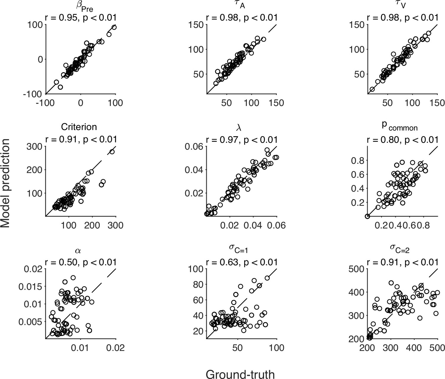
Predicted value vs. simulated value of each parameter.
Each dot represents 1 out of 100 simulated datasets. The identity line marks perfect recovery performance.
Tables
Table 1
Model parameters.
Check marks signify that the parameter is used for determining the likelihood of the data from the temporal-order judgment task in the pre- and post-test phase and/or for the Monte Carlo simulation of recalibration in the exposure phase.
| Notation | Specification | Temporal-order- judgment task | Recalibration in the exposure phase |
|---|---|---|---|
| The fixed relative delay between visual and auditory processing, i.e., the audiovisual bias prior to the exposure phase | |||
| Amount of auditory latency noise, the exponential time constant of the auditory arrival-latency distribution | |||
| Amount of visual latency noise, the exponential time constant of the visual -latency distribution | |||
| The spread of the Gaussian prior for the common-cause scenario | |||
| The spread of the Gaussian prior for the separate-causes scenario | |||
| The prior probability of a common cause | |||
| Simultaneity criterion | |||
| λ | Lapse rate | ||
| α | Learning rate for shifting audiovisual bias |
Appendix 6—table 1
Parameter estimates of individual participants.
All parameters except , and α are in milliseconds.
| Criterion | λ | α | |||||||
|---|---|---|---|---|---|---|---|---|---|
| S1 | –66.78 | 49.76 | 67.89 | 91.74 | 0.005 | 0.671 | 0.003 | 69.51 | 214.24 |
| S2 | 45.86 | 90.41 | 144.48 | 185.86 | 0.047 | 0.498 | 0.007 | 70.66 | 390.54 |
| S3 | 10.94 | 94.48 | 86.64 | 190.74 | 0.008 | 0.504 | 0.007 | 40.05 | 260.65 |
| S4 | –4.42 | 80.78 | 113.14 | 105.57 | 0.054 | 0.221 | 0.014 | 17.99 | 267.67 |
| S5 | 30.15 | 89.35 | 66.38 | 109.35 | 0.049 | 0.571 | 0.004 | 69.53 | 263.09 |
| S6 | –9.79 | 41.69 | 62.88 | 85.54 | 0.029 | 0.345 | 0.006 | 69.71 | 528.98 |
| S7 | –31.37 | 68.79 | 60.78 | 59.69 | 0.051 | 0.864 | 0.002 | 18.57 | 218.73 |
| S8 | 0.16 | 66.37 | 76.78 | 63.25 | 0.017 | 0.378 | 0.008 | 26.48 | 247.67 |
| S9 | 14.03 | 33.22 | 41.23 | 47.12 | 0.014 | 0.632 | 0.007 | 73.70 | 575.44 |
| Mean | –1.25 | 68.32 | 80.02 | 104.32 | 0.031 | 0.520 | 0.006 | 50.69 | 329.67 |
| SEM | 11.10 | 7.51 | 10.41 | 17.32 | 0.007 | 0.064 | 0.001 | 8.16 | 45.53 |
| Lower bound | –200 | 10 | 10 | 1 | 0 | 0 | 0 | 1 | 100 |
| Upper bound | 200 | 200 | 200 | 350 | 0.06 | 1 | 0.02 | 300 | 1000 |
Additional files
Download links
A two-part list of links to download the article, or parts of the article, in various formats.
Downloads (link to download the article as PDF)
Open citations (links to open the citations from this article in various online reference manager services)
Cite this article (links to download the citations from this article in formats compatible with various reference manager tools)
Precision-based causal inference modulates audiovisual temporal recalibration
eLife 13:RP97765.
https://doi.org/10.7554/eLife.97765.3


