Diverse prey capture strategies in teleost larvae
- Max Planck Institute for Biological Intelligence, Department Genes – Circuits – Behavior, Germany
Figures
Figure 1 with 7 supplements
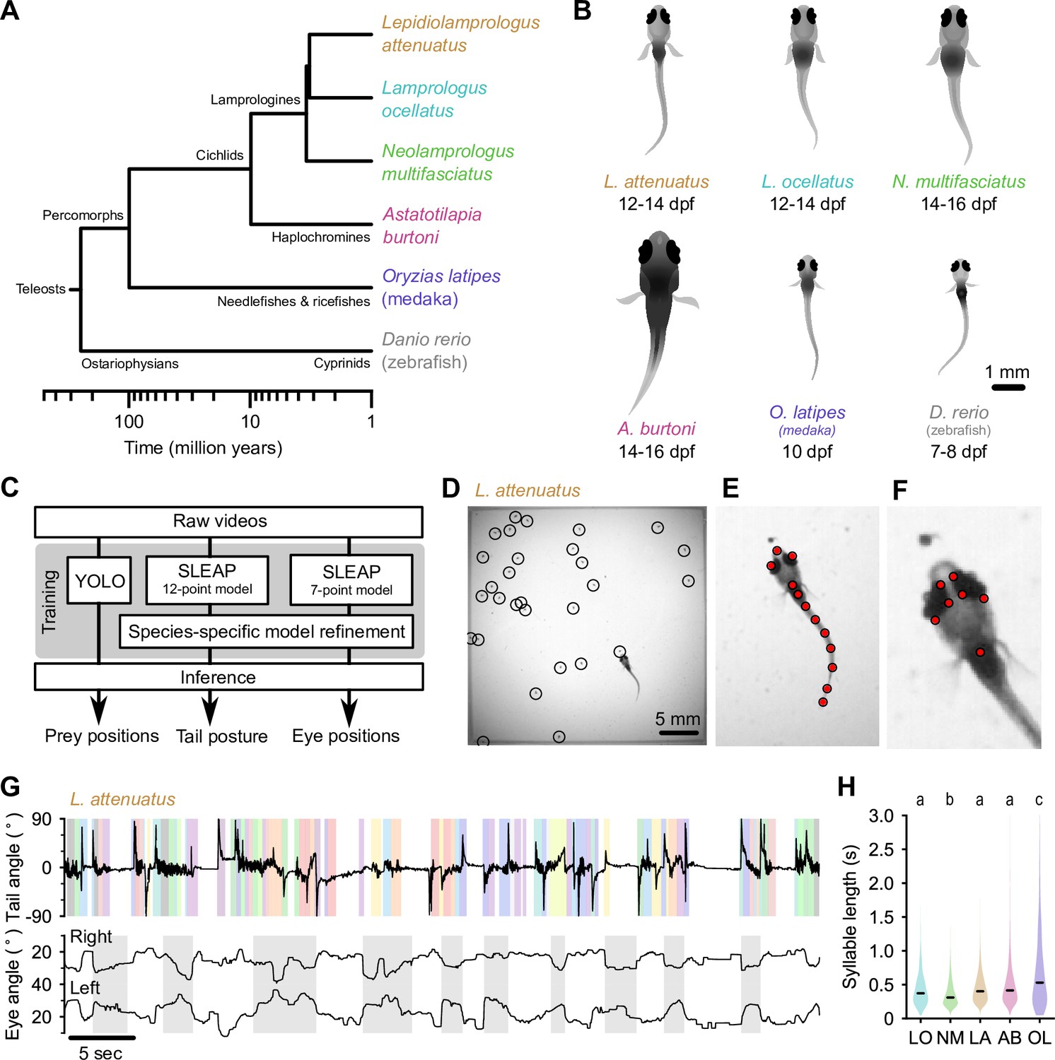
Tracking prey capture behavior in five species of fish larvae.
(A) Phylogenetic relationship between percomorph species used in this study and their relationship to zebrafish (a cyprinid). Based on Betancur-R et al., 2017. (B) Schematics of larvae of each species studied here (and zebrafish, Danio rerio, for reference). Scale bar: 1 mm. (C) Outline of tracking procedure. Raw video frames were analyzed with three different neural networks to extract tail pose, eye pose, and prey position in each frame. Kinematic features were extracted from raw pose data and used for subsequent analyses. (D–F) Tracking output for each neural network for a single frame from a recording of a Lepidiolamprologus attenuatus larva, showing identified artemia (D), tail points (E), and eye points (F). (G) One minute of tail and eye tracking from L. attenuatus showing tail tip angles (top trace) and right and left eye angles (bottom traces) relative to midline. Bottom trace, gray shaded boxes: automatically identified prey capture periods, when the eyes are converged (see Figure 3). Top trace, shaded boxes: automatically identified and classified behavioral syllables. Color corresponds to cluster identity in Figure 5. (H) Distribution of syllable length across species for all fish combined. Black bars indicate median; letters denote significance groups (bootstrap test difference between medians with Bonferroni correction). See also Figure 1—figure supplement 1.
Figure 1—figure supplement 1
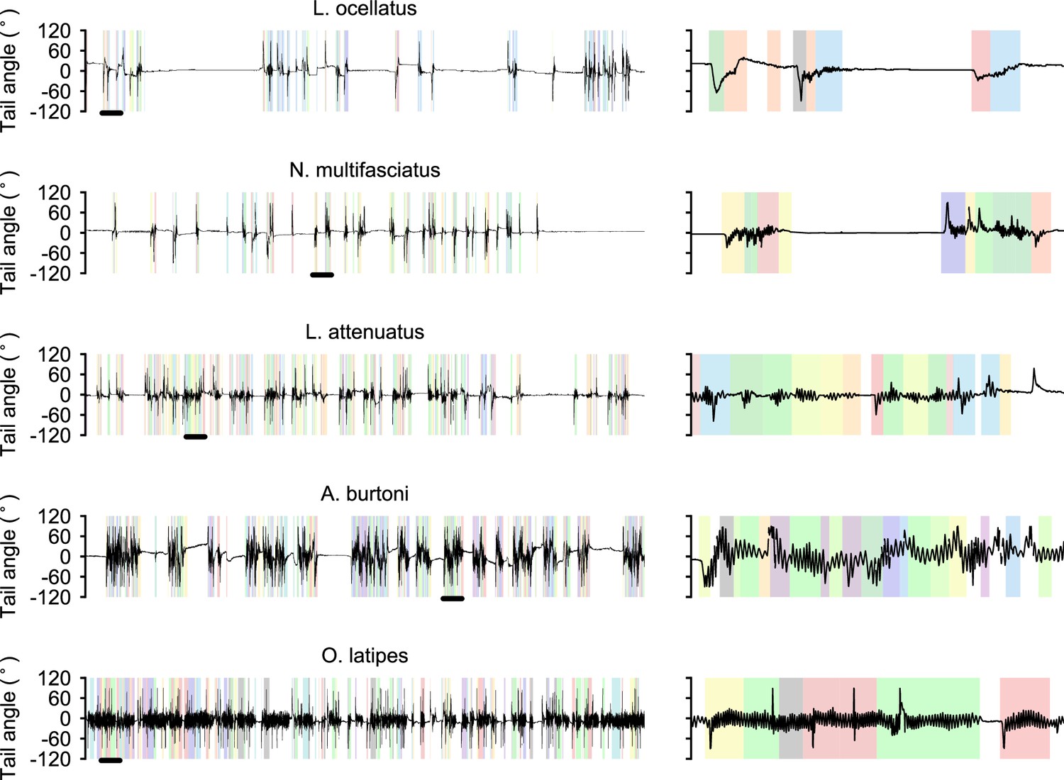
Diversity of swimming behavior in teleost larvae.
Left: representative 5 min of swimming from each species. Black bar indicates a 10 s window expanded on the right. Colors indicated automatically segmented and classified bouts within each swimming episode.
Figure 1—video 1
Pose tracking in freely swimming L. attenuatus, slowed ×10.
Tail points are shown in red, and eye points are shown in cyan.
Figure 1—video 2
Example of L. attenuatus freely swimming and hunting artemia, played at half speed.
Figure 1—video 3
Example of L. ocellatus freely swimming and hunting artemia, played at half speed.
Figure 1—video 4
Example of Neolamprologus multifasciatus freely swimming and hunting artemia, played at half speed.
Figure 1—video 5
Example of Astatotilapia burtoni freely swimming and hunting artemia, played at half speed.
Figure 1—video 6
Example of medaka (O. latipes) freely swimming and hunting paramecia, played at half speed.
Notice the side swings of the head during prey capture and the lack of eye convergence.
Figure 2
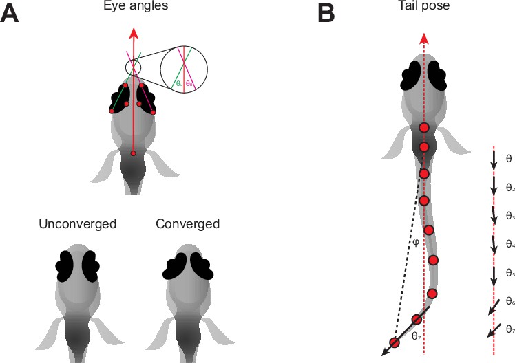
Pose information extracted from tracking data.
(A) Definition of left (θL) and right (θR) eye vergence angles. The heading vector (red arrow) is the vector starting from the midpoint of the fins and passing through the midpoint of the eyes. The orientation of each eye is computed from the temporal and nasal points (long axis of the eye). The eye angle is the signed angle between the heading and long axis of the eye. Zero degrees indicates that the long axis of the eye is parallel with the heading. Nasalward rotation of the eye increases the vergence angle. Eye convergence angle is θL + θR. Bottom: schematic showing eyes in an unconverged and converged state. (B) Parameters used to estimate tail pose. Tail pose is measured starting from the middle of the swim bladder. We compute the vector between each consecutive pair of points along the tail. At each pair of points, we compute the signed angle between the corresponding vector and the midline of the fish (RHS: θ1-7, angles between black arrows and red dashed line), providing a seven-dimensional representation of the tail pose in each frame. For visualization purposes in Figure 1G, Figure 1—figure supplement 1, we plot the tail angle, which is the signed angle between the swim bladder and the final tail point relative to the heading (angle between dashed red and black lines, φ).
Figure 3 with 1 supplement
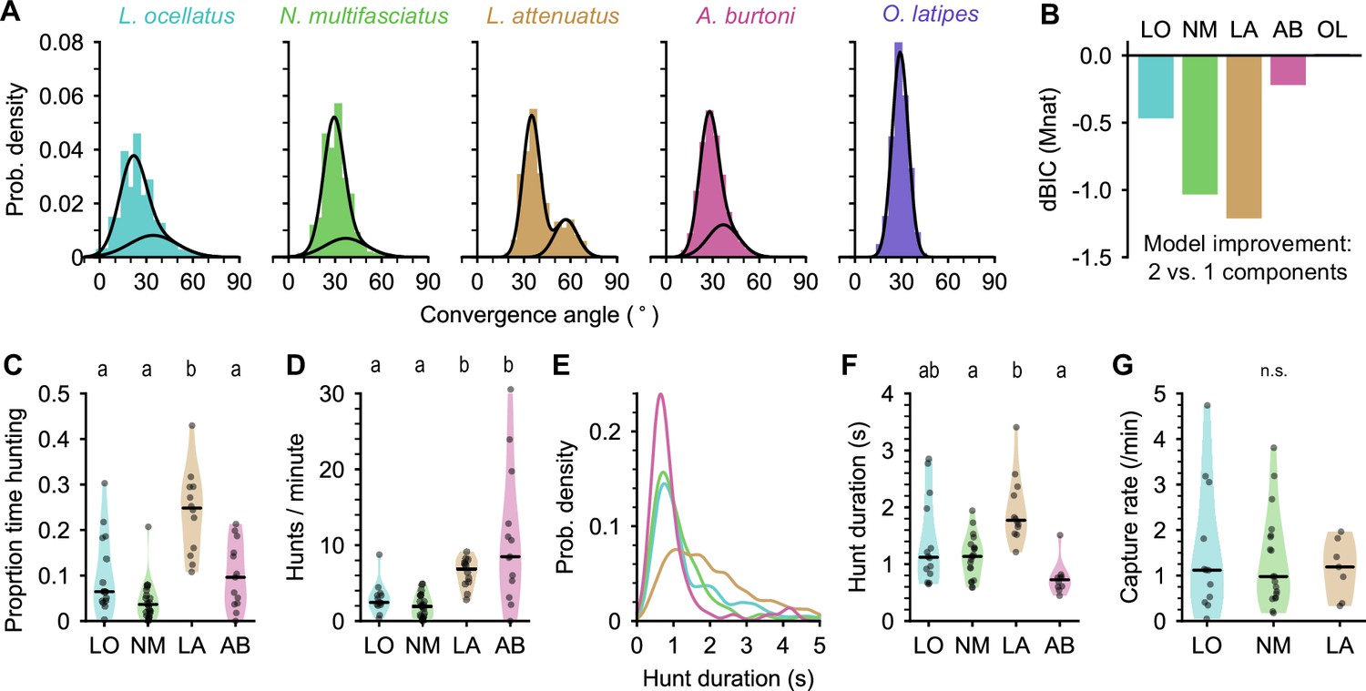
Eye movements during prey capture and statistics of hunting sequences.
(A) Histograms of eye convergence angles for each species. The convergence angle is the angle between the long axes of the eyes. Shaded bars: normalized binned counts of convergence angles from all fish. Black lines: a best fit Gaussian mixture model for each species (with one or two components). For all cichlid species, the data are better modeled as being drawn from two underlying distributions. For medaka (O. latipes [OL]), the data are better modeled with a single underlying distribution. (B) Improvement in fit for a two-component over single-component Gaussian mixture model, assessed using Bayesian inference criterion (BIC). The BIC is a measure of model fit, while punishing over-fitting. Lower values are better. Two mixtures provide a better fit over a single mixture for all species except medaka (OL). (C) Proportion of time spent by cichlids engaged in prey capture within the first 5 min of being introduced to the behavior arena. Points are single animals; black bar is the median; letters indicate significance (different letters indicate difference between groups, α=0.05). (D) Hunting rate, measured as the number of times eye convergence is initiated per minute, within the first 5 min. Points are single animals; black bar is the median; letters indicate significance. (E) Kernel density estimation of hunt durations for each species (all animals pooled). A. burtoni (pink) hunts skew shorter, L. attenuatus (brown) hunts tend to be longer. (F) Median hunt duration for each animal compared across species. Black bar is the median across animals; letters indicate significance. (G) Capture rate (number of artemia consumed) per minute over the first 5 min for three cichlid species. Black bar is the median across animals. n.s., no statistically significant difference between groups.
Figure 3—figure supplement 1
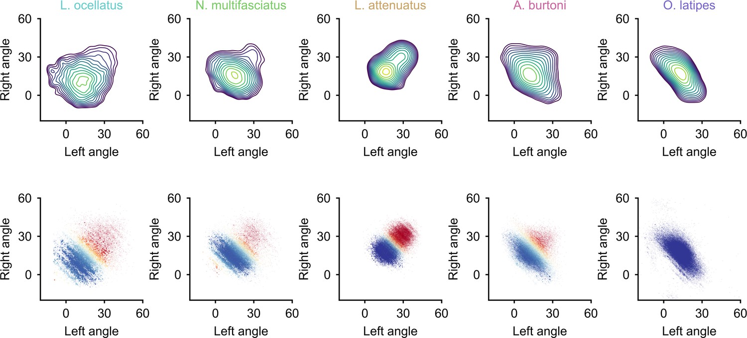
Two-dimensional (2D) histograms of eye angles.
Each point represents the angle of the left and right eyes in a given frame. Color corresponds to the probability a point belongs to a convergent state (red: converged; blue: not converged; yellow: equal likelihood).
Figure 4

Location of prey in the visual field during prey capture in cichlids.
(A) Trajectories of prey in the visual field for all automatically identified and tracked hunting events. Each prey is represented by a single line that changes in color from blue to yellow from the onset of eye convergence to when the eyes de-converge (end). Middle indicates the midpoint between eye convergence onset and end. Scale bar: 5 mm. (B) Kernel density estimation of the distribution of prey in the visual field across all hunting events. Rows: individual species. Columns: snapshots showing the distribution of hunted prey items at the beginning, middle, and end of hunting sequences. Scale bar: 2 mm. (C, D) Kernel density estimation of prey distance (C) and azimuthal angle from the midline (D) at the onset (top), in the middle (center), and at the end (bottom) of hunting episodes. Each column shows the distribution of all events for a single species.
Figure 5 with 3 supplements
Interspecies comparison of prey capture strategies.
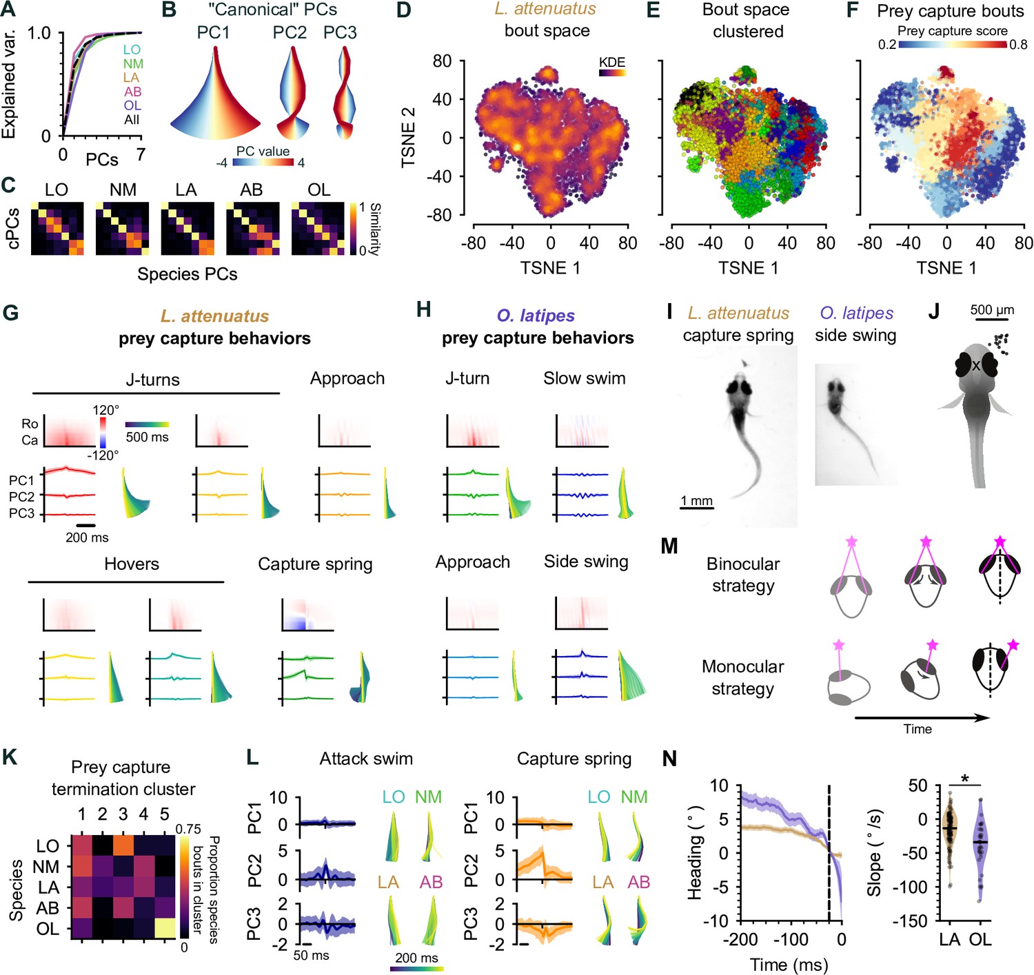
(A) Cumulative explained variance for the ‘canonical’ principal components (PCs) obtained from all species (black dotted line) and PCs for each species individually (colored lines). In all cases, three PCs explain >90% of the variance in tail shape. (B) ‘Eigenfish‘ of the first three canonical PCs. Each PC represents a vector of angles from the base to the tip of the tail (oriented with the fish facing up). At a given moment, the shape of the tail can be described as a linear combination of these vectors. Colors correspond to the tail shape obtained by scaling each PC from –4 to 4 standard deviations from the mean. (C) Each species’ eigendecomposition compared against the canonical PCs computed for all species together. Color intensity represents the cosine similarity between pairs of vectors. The strong diagonal structure (particularly in the first three PCs) shows that similar PCs are obtained by analyzing species separately or together. (D) Behavioral space of L. attenuatus (LA). Each point represents a single bout. Bouts are projected onto the first three PCs, aligned to the peak distance from the origin in PC space and then projected into a two-dimensional space using t-distributed stochastic neighbor embedding (t-SNE). Color intensity represents the density of surrounding points in the embedding. (E) Clustered behavioral space of LA. Clusters (colors) are computed via affinity propagation independently of the embedding. (F) Prey capture and spontaneous bouts in LA. Prey capture score is the probability that the eyes are converged at the peak of each bout. Bouts are colored according to the mean prey capture score for their cluster. Blue: clusters of bouts that only occur during spontaneous swimming; red: clusters of bouts that only occur during prey capture. (G, H) Example prey capture clusters from LA (G) and medaka, O. latipes (OL) (H). For each cluster, top left: mean rostrocaudal bending of the tail over time; bottom left: time series of tail pose projected onto first three PCs (mean ± standard deviation); bottom right: reconstructed tail shape over time for mean bout. (I) Representative frames of an LA capture spring (left) and OL (medaka) side swing (right), highlighting differences in tail curvature between these behaviors. (J) Location of prey in the visual field (black dots) immediately prior to the onset of a side swing. All events mirrored to be on the right. X marks the midpoint of the eyes, aligned across trials. (K) Comparison of clustered hunt termination bouts from all species. Termination bouts from all species were sorted into five clusters based on their similarity. Rows show the proportion of bouts from each species that were assigned to each cluster (columns). Cichlid bouts are mixed among multiple clusters, while medaka bouts (OL) mostly sorted into a single cluster. (L) Capture strikes in cichlids. Representative examples of tail kinematics during attack swims (left) and capture springs (right) from each species, including time series of tail pose projected onto the first three PCs (mean ± standard deviation, all species combined) shown for each type of strike. (M) Two hypotheses for distance estimation make different predictions of how heading (black dotted line) changes over time as fish approach prey (pink star). Top: fish maintain prey in the central visual field and use binocular cues to judge distance. Bottom: fish ‘spiral’ in toward prey, using motion parallax to determine distance. Black arrows indicate motion of prey stimulus across the retina. (N) Change in heading over time leading up to a capture strike for LA (brown, n=113) and medaka (OL, purple, n=36). Left: time series of heading. Zero degrees represents the heading 25 ms prior to the peak of the strike (black dotted line). Mean ± s.e.m. across hunting events. Right: comparison of the rate of heading change, computed as the slope of a line fit to each hunting event 200–25 ms prior to the peak of the strike. The heading decreases more rapidly, leading up to a strike in medaka than in LA.
Figure 5—figure supplement 1
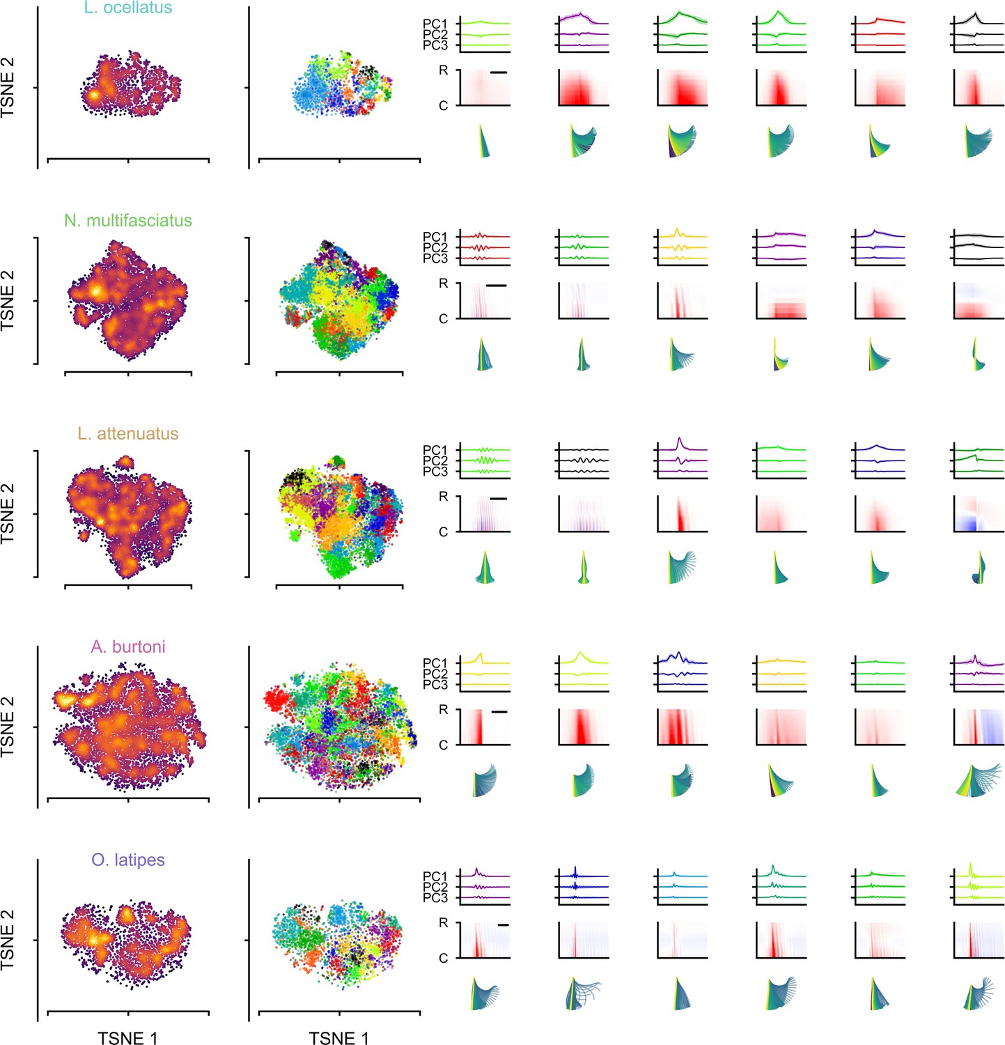
Behavioral spaces for each species.
Left: t-distributed stochastic neighbor embedding (t-SNE) embedding and cluster identity of automatically segmented bouts. Right: example clusters from each species, showing average time series in the first three principal components (PCs) (top), rostrocaudal tail bending (middle), and tail kinematics (bottom) for each cluster. For cichlids, behaviors on the right are more likely to occur during prey capture, and behaviors on the left are more likely to occur during spontaneous swimming.
Figure 5—video 1
L. attenuatus spitting behavior, played at half speed.
Figure 5—video 2
A. burtoni swimming backward during prey capture, played at half speed.
Figure 6
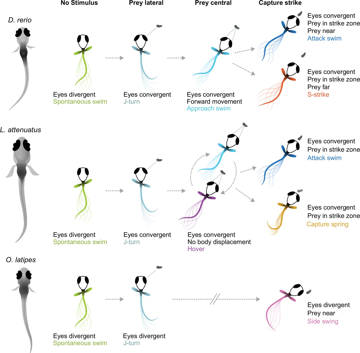
Schematic of hunting strategies in teleost larvae.
Top: prey capture in zebrafish larvae (D. rerio) begins with eye convergence and a J-turn to orient toward the prey. The prey is then approached with a series of low-amplitude approach swims. Once in range in the central visual field, the prey is captured with an attack swim or an S-strike. Middle: prey capture in cichlids (represented by L. attenuatus) also begins with eye convergence and a J-turn. Prey is approached with a wide variety of tail movements. The prey is captured when it is in the central visual field with either an attack swim or a capture spring, during which the tail coils over several hundreds of milliseconds. Bottom: prey capture in medaka (O. latipes) begins with reorienting J-like turns, but these do not centralize prey in the visual field. Instead, the prey is kept lateral in the visual field and is captured with a side swing.
Tables
Key resources table
| Reagent type (species) or resource | Designation | Source or reference | Identifiers | Additional information |
|---|---|---|---|---|
| Biological sample (Lamprologus ocellatus) | LO | Other | From Alex Jordan, Max Planck Institute of Animal Behavior, Konstanz | |
| Biological sample (Neolamprologus multifasciatus) | NM | Bose et al., 2020 | From Alex Jordan, Max Planck Institute of Animal Behavior, Konstanz | |
| Biological sample (Lepidiolamprologus attenuatus) | LA | Other | From Alex Jordan, Max Planck Institute of Animal Behavior, Konstanz | |
| Biological sample (Astatotilapia burtoni) | AB | Other | From Alex Jordan, Max Planck Institute of Animal Behavior, Konstanz | |
| Biological sample (Oryzias latipes –wild-type) | Medaka; OL | Other | From Joachim Wittbrodt, University of Heidelberg | |
| Software | SLEAP | Pereira et al., 2019; Pereira et al., 2022 | Social LEAP Estimates Animal Pose | |
| Software | YOLO | Redmon et al., 2016 | You Only Look Once | |
| Software, algorithm | Python code | Mearns et al., 2020 | Python code | |
| Software, algorithm | Custom analysis code (Python 3) | GitHub, copy archived at Mearns, 2025 | Custom analysis code (Python 3) |
Additional files
Download links
A two-part list of links to download the article, or parts of the article, in various formats.
Downloads (link to download the article as PDF)
Open citations (links to open the citations from this article in various online reference manager services)
Cite this article (links to download the citations from this article in formats compatible with various reference manager tools)
Diverse prey capture strategies in teleost larvae
eLife 13:RP98347.
https://doi.org/10.7554/eLife.98347.3


