Sub-type specific connectivity between CA3 pyramidal neurons may underlie their sequential activation during sharp waves
- Charité-Universitätsmedizin Berlin, corporate member of Freie Universität Berlin and Humboldt-Universität zu Berlin, Neuroscience Research Center, Germany
- Institute for Theoretical Biology, Department of Biology, Humboldt-Universität zu Berlin, Germany
- Bernstein Center for Computational Neuroscience, Germany
- Charité-Universitätsmedizin Berlin, corporate member of Freie Universität Berlin and Humboldt-Universität zu Berlin, Einstein Center for Neurosciences, Germany
- German Center for Neurodegenerative Diseases (DZNE), Germany
- Max-Delbrück Center for Molecular Medicine in the Helmholtz Association, Germany
- Charité – Universitätsmedizin Berlin, corporate member of Freie Universität Berlin and Humboldt-Universität zu Berlin, NeuroCure Cluster of Excellence, Germany
Figures
Figure 1 with 1 supplement
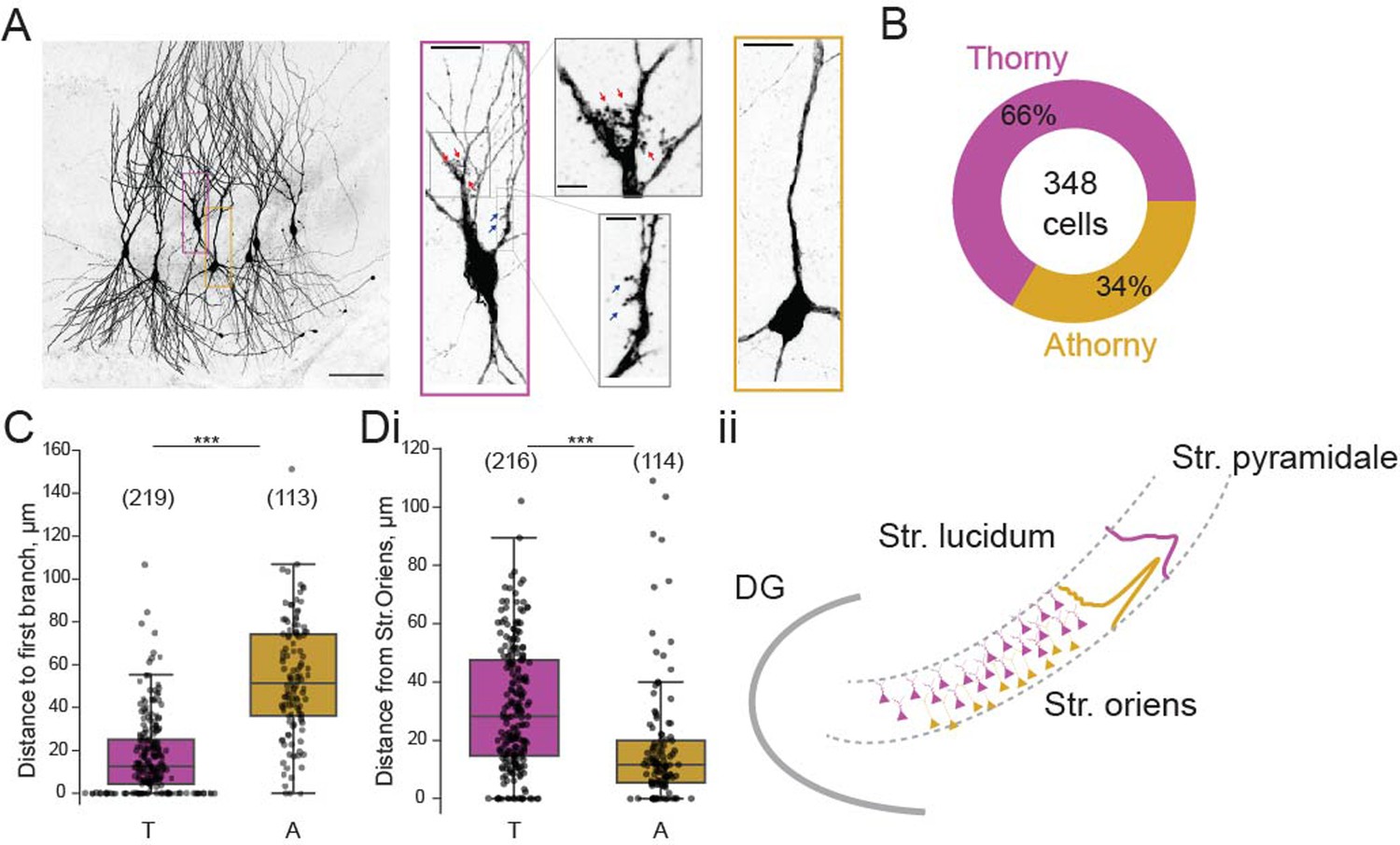
Proportion and distribution of thorny and athorny pyramidal neurons in CA3.
(A) Left, image of seven pyramidal neurons recorded simultaneously and filled with biocytin to reveal thorny and athorny morphologies. Right, the magenta box contains a typical example of a thorny CA3 pyramid, gray boxes show close-ups of regions with thorns; yellow box shows a typical athorny pyramidal neuron. Scale bar in left image 100 µm, in magenta/yellow boxed insets 20 µm, in gray boxed insets 5 µm. (B) Proportion of thorny and athorny cells in total recorded pyramidal neurons. (C) Distance from soma to the first branch point for thorny (T) and athorny (A) CA3 pyramidal neurons. (Di) Location of thorny and athorny cell somata across the deep-superficial axis of the pyramidal layer. N numbers for each group shown above boxplots in parentheses. (Dii) Schematic depicting the distribution of thorny and athorny pyramids in the deep-superficial axis of the CA3 pyramidal layer.
Figure 1—figure supplement 1

Intrinsic properties of thorny (T) and athorny (A) cells.
Significance calculated using Mann-Whitney U and corrected for multiple comparisons. *** *; For thorny n=185; for athorny n = 103.
Figure 2
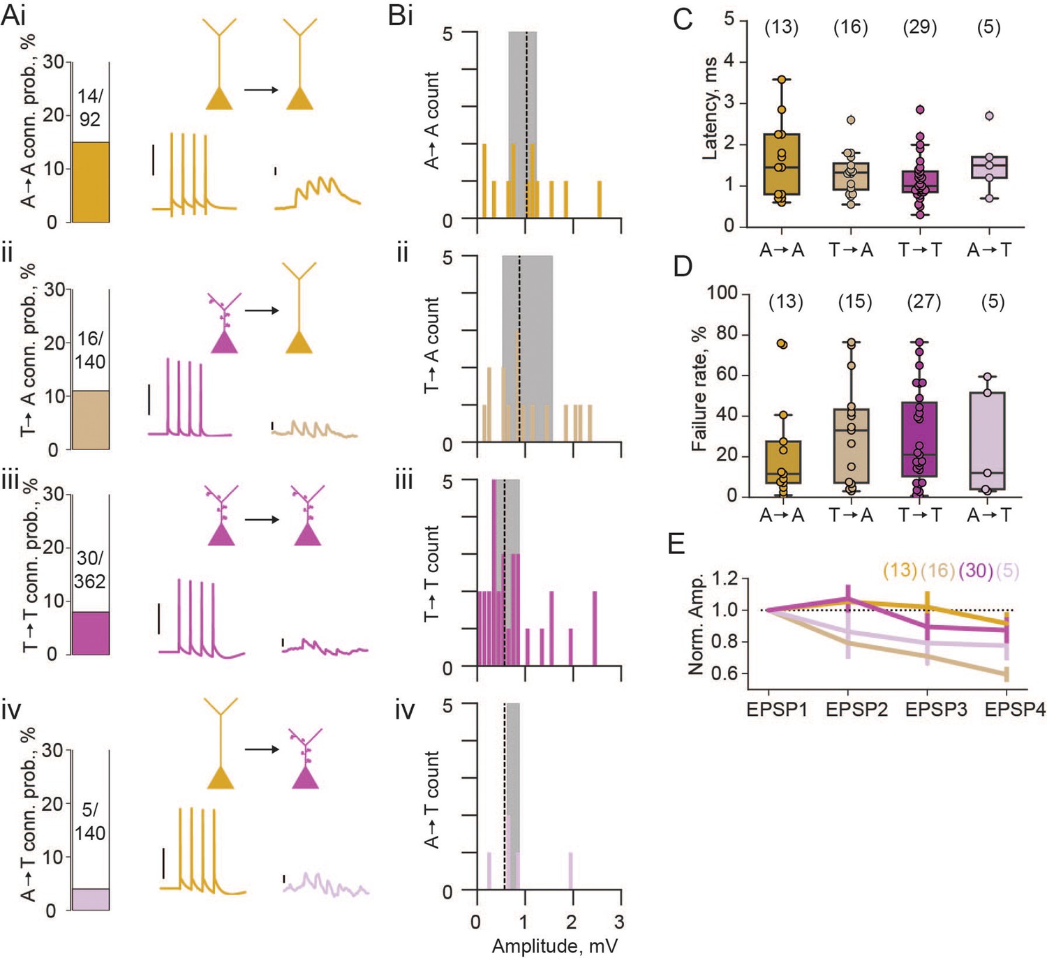
Properties of excitatory connections between athorny (A) and thorny (T) CA3 pyramids.
(A) Connection probabilities (conn. prob.) and example connections: i, from A to A cells (A→A); ii, T→A; iii, T→T; iv, A→T. Scalebars for presynaptic action potentials, 40 mV; for postsynaptic responses, 0.5 mV. (B) Histograms of synaptic amplitudes of the different connection types. Dashed lines represent median values and shaded areas interquartile ranges. (C) Latency of different synaptic connection types, individual points show single connection values. (D) Failure rates of the different synaptic connection types. (E) Short-term plasticity dynamics of different synaptic connection types. Synaptic amplitudes are normalised to the first EPSP in the train of 4 and plotted as mean ± s.e.m. N numbers for groups shown above plots in parentheses.
Figure 3
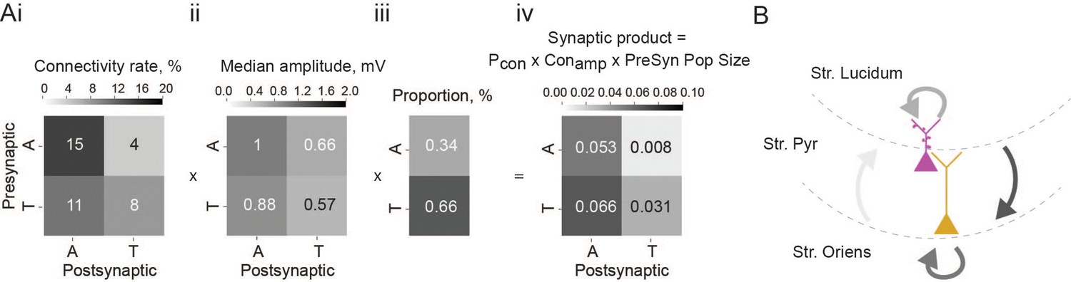
Summary of overall impact of each connection type.
(Ai) Matrix showing connection rates between the four combinations of connection types, ii, matrix showing mean connection strength for the four connection types, iii, proportion of each cell type found in the CA3 pyramidal population, iv, matrix showing the synaptic product, calculated as the product of the matrices in i and ii multiplied by the presynaptic population size shown in iii. (B) Schematic depicting the connections between the two pyramidal cell types in the CA3, line colour is coded by connection impact.
Figure 4 with 3 supplements
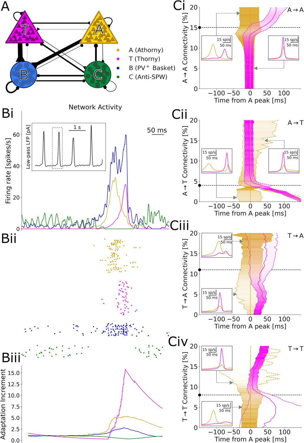
Results of numerical simulations.
(A) Network scheme. (Bi) Firing rates before, during, and after a sharp wave-ripple complex (SPW). Inset: low-pass filtered estimate of the LFP over a longer window of 10 s. ii, Spike raster plot of a representative sample of each neuron type. iii, Relative increment of the average adaptive currents received by each population with respect to a 200 ms baseline before the event. (C) Effects of varying each connectivity from its default value, marked by a black dashed line and dot. Continuous gold/magenta lines indicate the peak time of each population rate (with the peak of A always plotted at 0), while dashed ones represent the time at which the rate equals 25% of the respective peak. The peak size for each connectivity value is color-coded. In these simulations, the synaptic strengths of all the excitatory-to-excitatory synapses were up- or down-scaled by a common factor, in order to obtain SPW events with a comparable size (measured based on the activity of B interneurons, see Materials and Methods). Insets: firing trace of each population averaged over many events, for particular connectivity values highlighted by the gray arrows.
Figure 4—figure supplement 1

Onset f-I curves for each neuron type, calculated, for comparability, by delivering a constant current for 500 ms, like in Hunt et al., 2018.
These curves (colored solid lines) are compared to experimental data (black dots) from Hunt et al., 2018 for A and T neurons, and from Fidzinski et al., 2015 for B neurons. Dashed lines represent transient firing. Insets: example of firing patterns displayed by the different neurons in response to the specific current values marked by vertical gray lines in the main figure.
Figure 4—figure supplement 2

Simulations with short-term synaptic depression.
Same as Figure 4, but excitatory–to–excitatory synapses are subject to short-term synaptic depression; for details, see Materials and methods. The model dynamics and the effects of excitatory-to-excitatory connections are qualitatively analogous.
Figure 4—figure supplement 3

Simulations with heterogeneity.
Same as Figure 4, but several parameters of thorny and athorny cells are sampled from Gaussian distributions centered around their mean, with a standard deviation based on the data in Figures 2B–C –1 (see Materials and methods). Compared to the results with the basic model, here peaks tend to be more spread out in time; however, increasing the A→A or decreasing the A→T connectivity still increases the delay between the peaks.
Figure 5 with 1 supplement
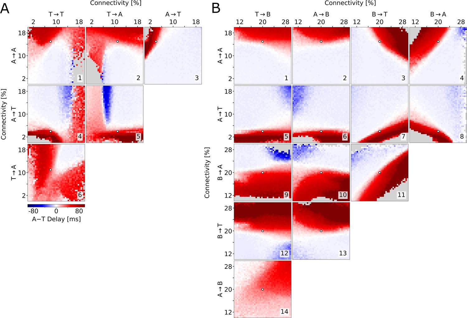
Exploration of the parameter space.
Average delay between the athorny and the thorny peak, as a function of two connectivity parameters (pairs of excitatory-to-excitatory connections in (A), pairs involving inhibitory connections in (B)). In each simulation, the connectivity rates were varied from their default value (marked by a white dot), while all the excitatory-to-excitatory synaptic strengths were scaled, as in Figure 4, in order to obtain sharp waves with a comparable size. Data points are plotted only if both populations exceed a lower threshold on the firing rate; otherwise, they are grayed out. The same simulations as in (A), but with a different scaling, are reported in Figure 5—figure supplement 1.
Figure 5—figure supplement 1

Alternative scaling.
Same as Figure 5A, but the size of sharp wave-ripple complex (SPW) events is maintained by up- or down-scaling of a common factor the synaptic strengths of A→B and T→B synapses, which in Figure 5B were found to be little relevant for the delay between the peaks. The main results are consistent between the two scalings, except that here it is easier to appreciate that T→T is little relevant for the peak delay, which in Figure 5A appears less clean due to the simultaneous scaling of all the excitatory-to-excitatory conductances.
Tables
Table 1
Single neuron parameters.
| Athorny (A) | Thorny (T) | PV+- Basket (B) | Anti-SPW (C) | ||
|---|---|---|---|---|---|
| Population size | 2700 | 5300 | 150 | 100 | |
| [pF] | 200 | 200 | 100 | 100 | |
| [nS] | 8 | 11 | 8 | 5 | |
| [mV] | –60 | –70 | –55 | –57 | |
| [mV] | –48 | –44 | –40 | –40 | |
| [mV] | –42 | –46 | –57 | –52 | |
| [nS] | 4 | 0 | 6 | 2.5 | |
| [pA] | 85 | 150 | 25 | 20 | |
| [ms] | 200 | 200 | 50 | 100 | |
| [ms] | 3 | 3 | 3 | 3 | |
| [mV] | 2.5 | 2.5 | 2.5 | 2.5 | |
| [pA] | 140 | 285 | 180 | 160 | |
Table 2
Network parameters.
Parameter adjustments for the model variants with short-term synaptic depression and heterogeneity are reported in Supplementary file 1.
| From A | From T | From B | From C | ||
|---|---|---|---|---|---|
| 15% | 11% | 20% | 20% | ||
| 4% | 8% | 20% | 20% | ||
| 20% | 20% | 20% | 20% | ||
| 20% | 20% | 20% | 20% | ||
| [nS] | 0.2 | 0.2 | 2.15 | 15 | |
| [nS] | 0.2 | 0.2 | 0.8 | 15 | |
| [nS] | 0.7 | 0.5 | 6 | 9 | |
| [nS] | 0.1 | 0.05 | 5 | 3 | |
| [ms] | 2 | 2 | 4 | 4 | |
| [mV] | 0 | 0 | –70 | –70 | |
| [ms] | 1 | 1 | 1 | 1 |
Additional files
-
MDAR checklist
- https://cdn.elifesciences.org/articles/98653/elife-98653-mdarchecklist1-v1.pdf
-
Supplementary file 1
Parameter adjustments for model variants.
- https://cdn.elifesciences.org/articles/98653/elife-98653-supp1-v1.tex
Download links
A two-part list of links to download the article, or parts of the article, in various formats.
Downloads (link to download the article as PDF)
Open citations (links to open the citations from this article in various online reference manager services)
Cite this article (links to download the citations from this article in formats compatible with various reference manager tools)
Sub-type specific connectivity between CA3 pyramidal neurons may underlie their sequential activation during sharp waves
eLife 13:RP98653.
https://doi.org/10.7554/eLife.98653.3


