Perturbation-response analysis of in silico metabolic dynamics revealed hard-coded responsiveness in the cofactors and network sparsity
- Universal Biology Institute, University of Tokyo, Japan
- Center for Biosystems Dynamics Research, RIKEN, Japan
Figures
Figure 1 with 4 supplements
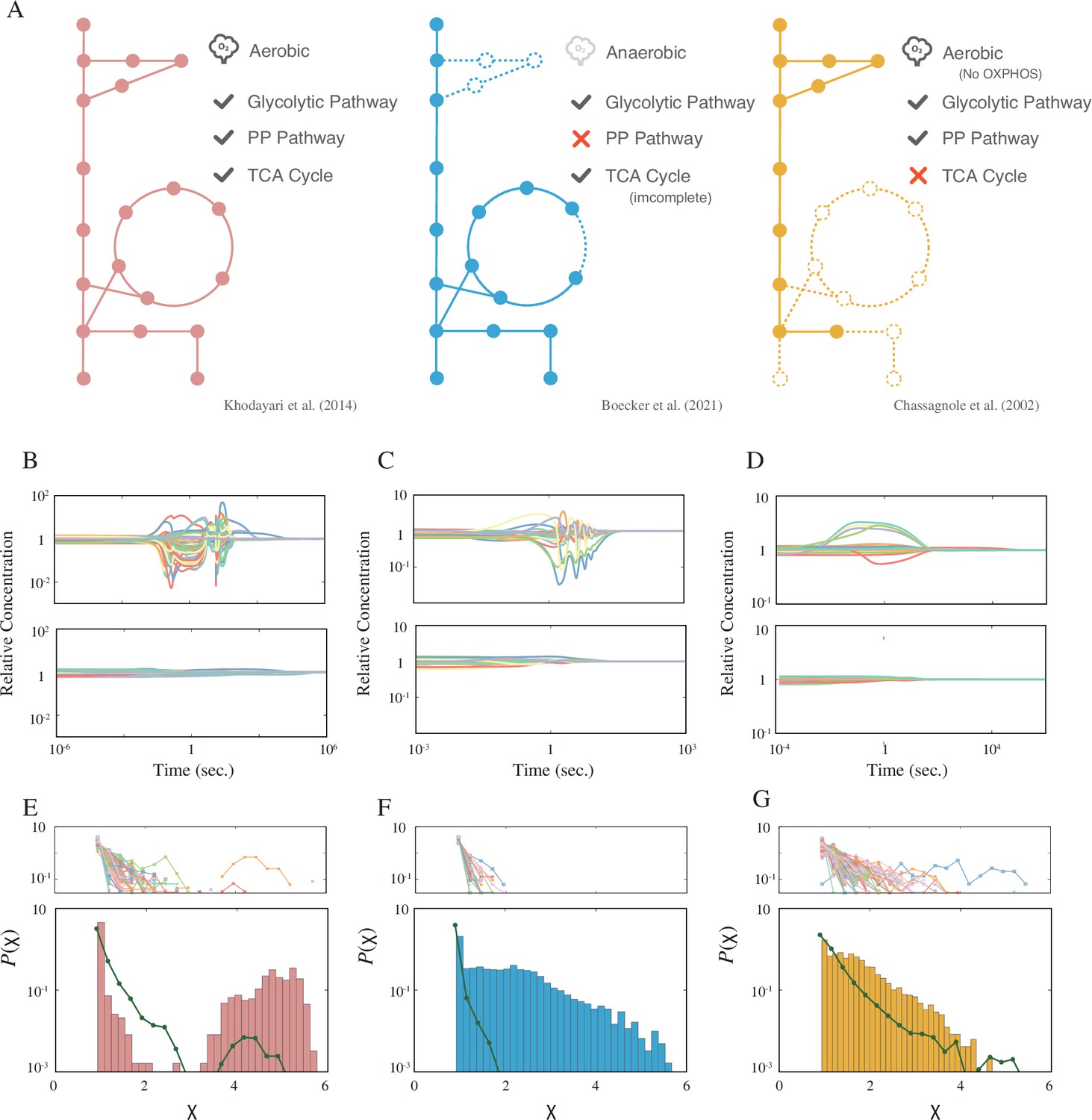
Models, dynamics, and distribution of the response coefficient.
(A) A graphical summary of the three models used in this study. The solid circles represent the metabolites, and the lines represent the metabolic reactions. The dashed circles and lines are the subsystems not implemented in the model. (B–D) Example time courses for each model. The top and bottom panels are examples of the strong and weak response, respectively. (E–G) The response coefficient distribution of each model (bottom). The average response coefficient distribution of the random catalytic reaction network (RCRN) model is overlaid (green line). The response coefficient distribution of each instance of the RCRN model is shown on the top panel. The model schemes, time courses, and distributions are aligned in each column, that is, the leftmost network of (A), (B), and (E) are from the model developed by Khodayari et al., 2014.
Figure 1—figure supplement 1
Scatter plot of the response coefficient.
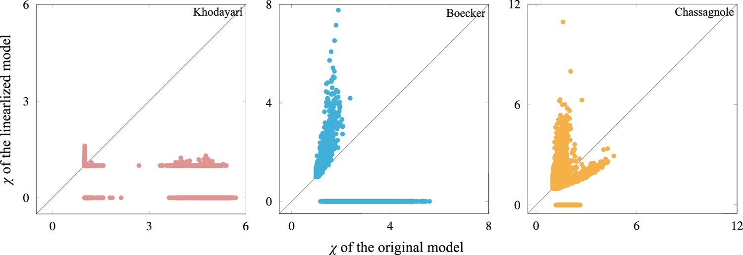
Each point corresponds to a single initial condition, while the horizontal and vertical axes represent the response coefficient computed by the original and the linearized model, respectively, around the steady state. The linearized model is given by , where is the Jacobi matrix of the model at steady state. If any metabolite concentrations become negative, the response coefficient is incomputable and ‘0’ is assigned to such trajectories (note that the minimum value of the response coefficient is unity). Since the response coefficient is based on the logarithm of the concentrations, as the metabolite concentrations approach zero, the response coefficient becomes larger. The high response coefficient in the Boecker and Chassagnole model will be explained by this artifact. The linearized Khodayari model shows either or (one or more metabolite concentrations become negative).This could be due to the number of variables in the model. For the response coefficient to have a larger value, the perturbation should be along the eigenvector that leads to oscillatory dynamics with long relaxation time (i.e., the corresponding eigenvalue has a small real part in terms of absolute value and a nonzero imaginary part). However, since the Khodayari model has about 800 variables, if perturbations are along such directions, there is a high probability that one or more metabolite concentrations will become negative.
Figure 1—figure supplement 2
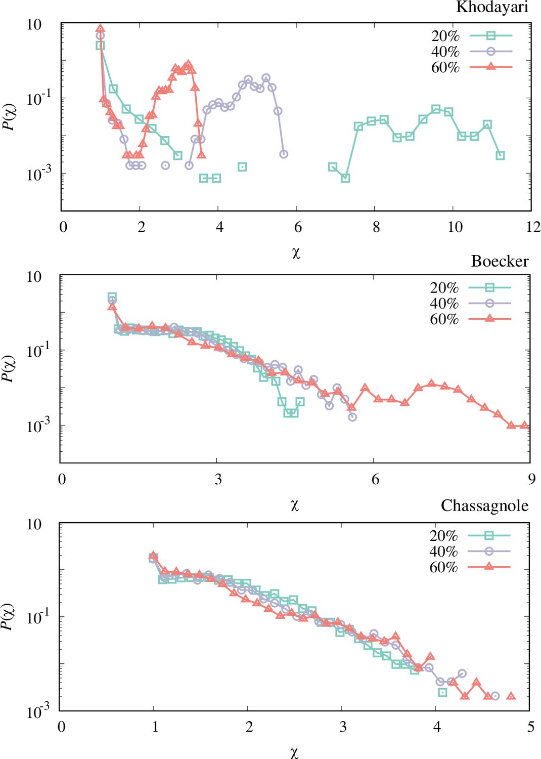
The response coefficient distribution of each model obtained by the perturbation-response simulation with different perturbation strengths (20%, 40%, and 60% relative perturbation).
Each distribution is obtained by simulating 4096 trajectories. The qualitative features (double-peaks for the Khodayari model and the plateau for the Boecker and Chassagnole models) are unvaried, while the scales of the response coefficient of the Khodayari model differ among the perturbation strengths.
Figure 1—figure supplement 3
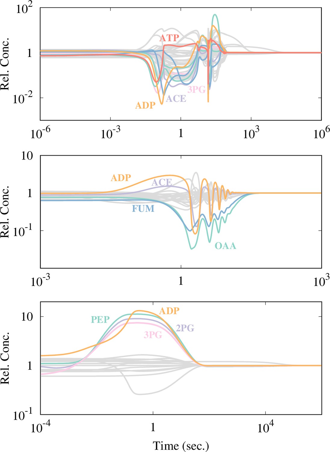
The time course of each model with the strongly responding metabolites being highlighted.
A metabolite is highlighted if its concentration changes more than -fold from its steady concentration. is set to be 5 for the Boecker and Chassagnole models, while is chosen for the Khodayari model because too many metabolites are highlighted with .
Figure 1—figure supplement 4

The response coefficient distribution of 215 realizations of the PYK model by the MASSpy framework (Himeoka et al., 2022a) is overlaied (each model has the same network structure, kinetic rate law, but the parameters are different).
For each model realization, we have computed 256 trajectories. Trajectories had negative value for any metabolites that are excluded for the computation of the distribution.
Figure 2 with 4 supplements
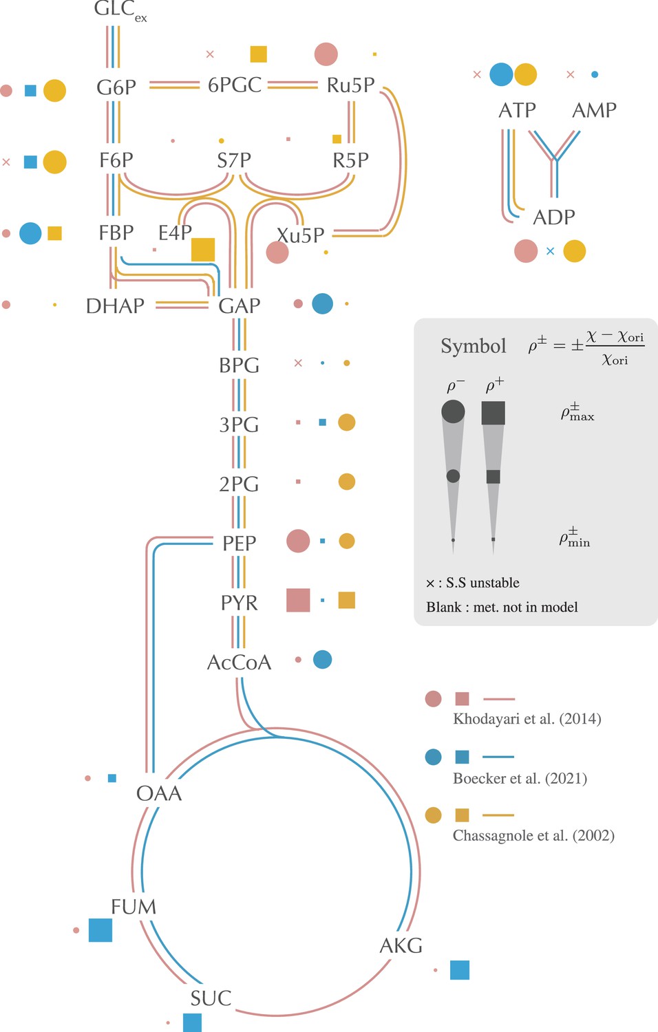
The impact of setting each metabolite’s concentration to its constant, and steady-state value is depicted on the metabolic network.
This impact is quantified by the relative change in the average response coefficient, as detailed in (1) and (2). The filled point and filled square symbols represent the decrease and the increase of the response coefficient, respectively. The size of the symbols is scaled using the maximum and minimum values of computed for each model. The cross symbol indicates that the original steady-state attractor becomes unstable when the concentration of the corresponding metabolite is fixed. If a dot, square, or cross is absent, the concentration of the corresponding metabolite is not a variable in the model. Only selected, representative metabolites are displayed in the figure. Comprehensive results are provided in Figure 2—figure supplement 1.
Figure 2—figure supplement 1
The average response coefficients of the models with the concentration of indicated metabolite fixed.
The dashed line in each panel is the average response coefficient of the original model.
Figure 2—figure supplement 2
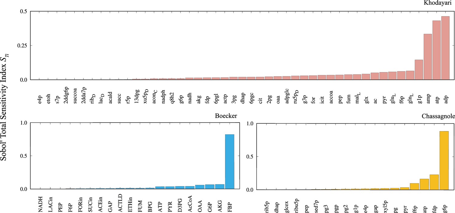
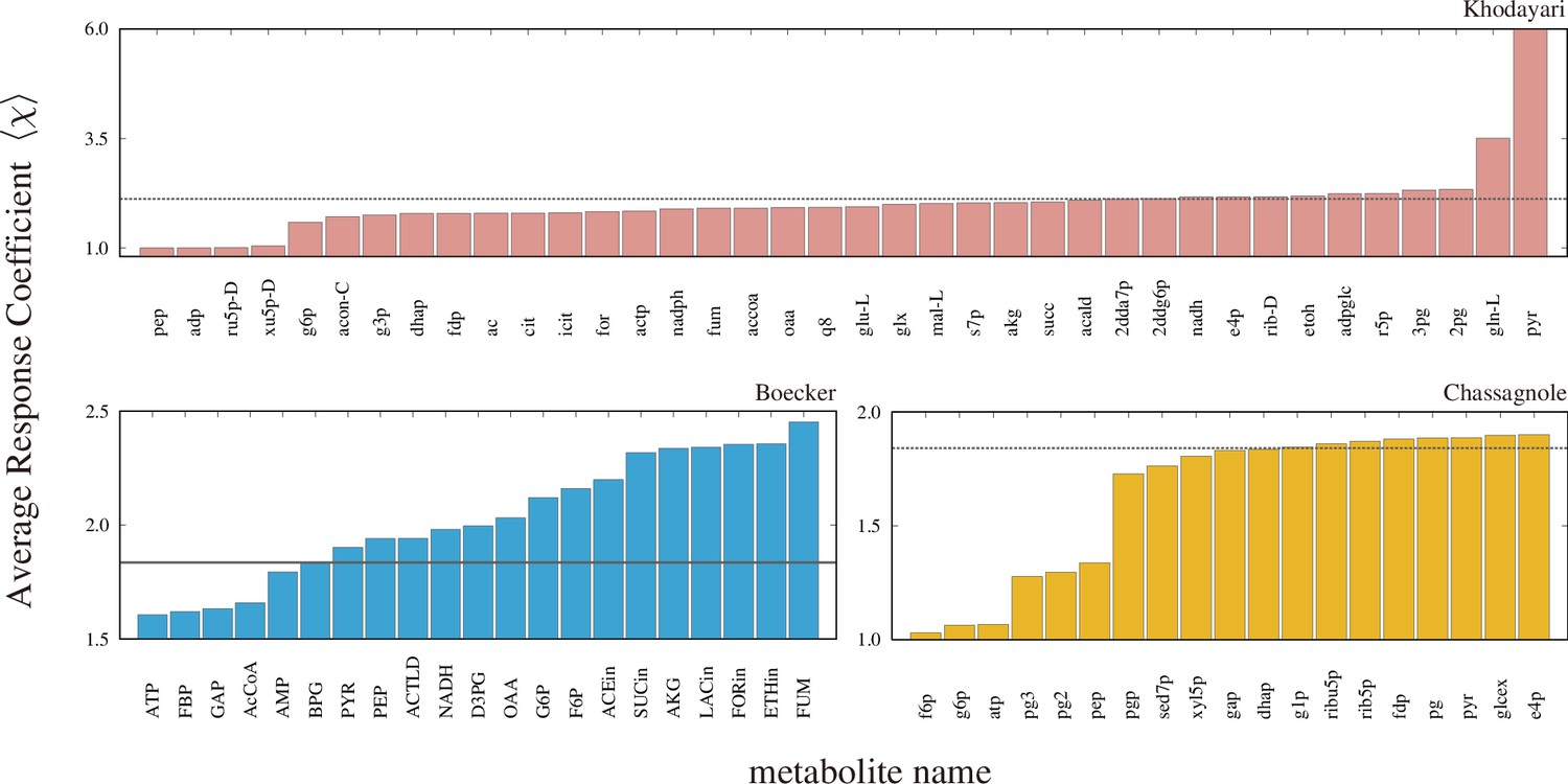
The Sobol’ total sensitivity index is computed for each metabolite.
The sensitivity indices are computed by simulating 512 trajectories for the Khodayari model and 4096 trajectories for the Boecker and Chassagnole models.
Figure 2—figure supplement 3
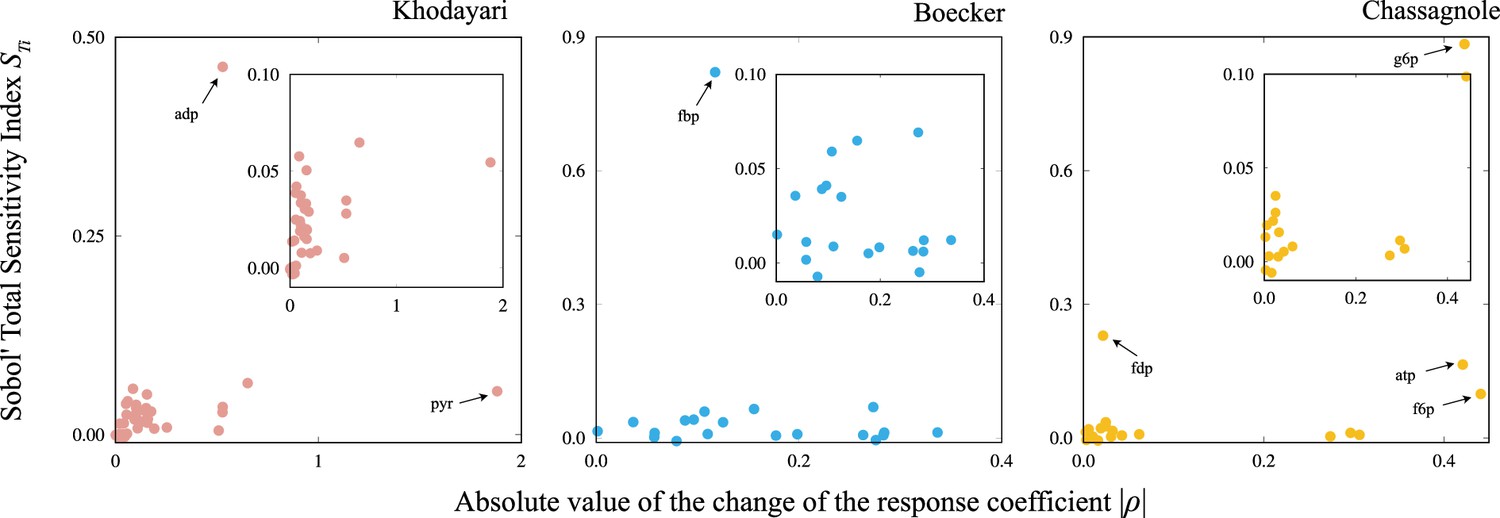
The scatter plot of the Sobol’ total sensitivity index versus the absolute value of the change in the response coefficient..
The inset presents a magnified view of a portion of each figure. The names of metabolites that deviate from the trend between and are highlighted.
Figure 2—figure supplement 4

The response coefficient distributions of models with weakened substrate-level regulation of enzyme activity.
The relaxations of the inhibition strength of AKG on CSICD and OAA on MDH increase the responsiveness of the model, while those of FUM on MDH and OAA on FRD have no effect. To relax the inhibition, the equilibrium constant for the corresponding competitive inhibition is set to (the inhibition term is implemented with the form in the denominator of the reaction rate function), where rxn, i, and met represent the reaction name, ‘inhibition’, and the metabolite name, respectively. Each distribution is computed from 4096 trajectories.
Figure 3 with 1 supplement
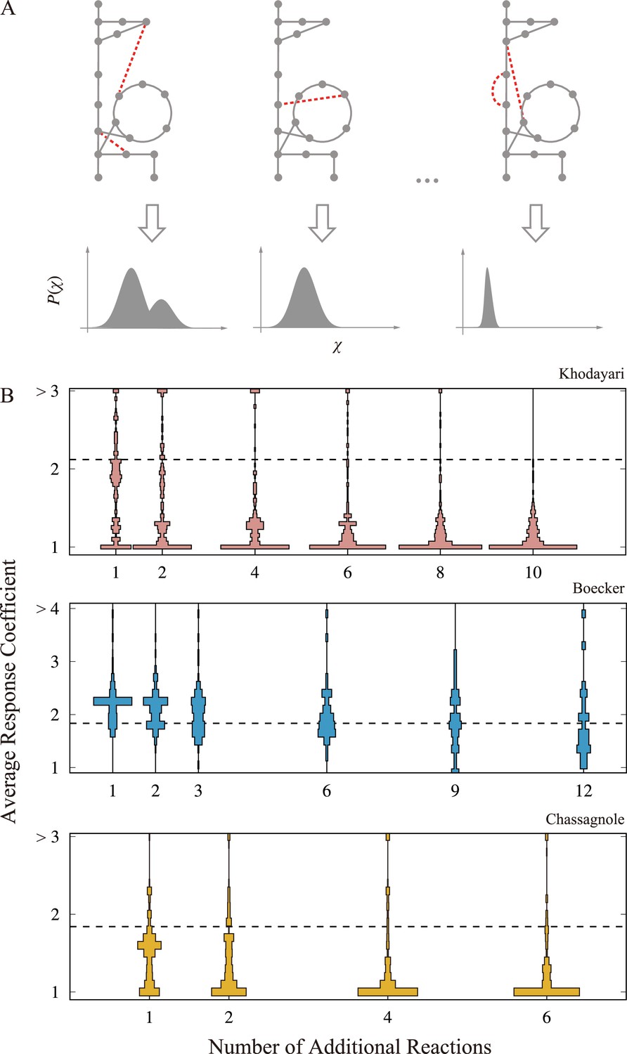
Change in the responsiveness by network expansion.
(A) A schematic figure of the network expansion simulation. Reactions are randomly added to the original metabolic network, and then, the corresponding ordinary differential equation (ODE) model is constructed. In the illustration, the additional reaction is highlighted as the dashed red lines. The perturbation-response simulation is performed on the expanded models to obtain the response coefficient distribution. The average response coefficient is calculated as a scalar indicator of the responsiveness for each response coefficient distribution. (B). The distribution of the average response coefficient is plotted against the number of additional reactions for the three models. The dashed line indicates the average response coefficient of the original model with no additional reaction. For each , we generated 256 extended network, and 128 trajectories were computed for each extended network.
Figure 3—figure supplement 1

The violin plot of the average response coefficient of the network expansion of the Khodayari model.
The horizontal axis represents the number of additional reactions. The additional reactions are chosen from the reactions registered in the metabolic model database (see Supplementary file 1d).
Figure 4

The distribution of the average response coefficient is plotted against the number of reactions, , for the model with metabolites plus three cofactors (the panels labeled as ‘Cofactor’) and metabolites without cofactors (the panel labeled as ‘Catalytic’).
For each combination of and , we generated 512 random networks and computed 128 trajectories for each of these networks. The inverse temperature is set at 10 for the cofactor version and 20 for the catalytic version. This is because the maximum chemical potential difference in the cofactor version is 2.0, but it is 1.0 in the catalytic version. The total concentrations of the cofactors are set to be unity.
Additional files
-
MDAR checklist
- https://cdn.elifesciences.org/articles/98800/elife-98800-mdarchecklist1-v1.docx
-
Supplementary file 1
The list of substrate-level regulations in each model and reactions used for the non-random network expansion.
- https://cdn.elifesciences.org/articles/98800/elife-98800-supp1-v1.xlsx
Download links
A two-part list of links to download the article, or parts of the article, in various formats.
Downloads (link to download the article as PDF)
Open citations (links to open the citations from this article in various online reference manager services)
Cite this article (links to download the citations from this article in formats compatible with various reference manager tools)
Perturbation-response analysis of in silico metabolic dynamics revealed hard-coded responsiveness in the cofactors and network sparsity
eLife 13:RP98800.
https://doi.org/10.7554/eLife.98800.4


