Muscarinic receptors mediate motivation via preparatory neural activity in humans
- Nuffield Department of Clinical Neuroscience, University of Oxford, United Kingdom
- Trinity College Institute of Neuroscience and Department of Psychology, Trinity College Dublin, Ireland
- Department of Experimental, Clinical and Health Psychology, Ghent University, Belgium
- Nuffield Department of Surgical Sciences, University of Oxford, United Kingdom
Figures
Figure 1 with 1 supplement

Trihexyphenidyl (THP) modulates saccadic measures.
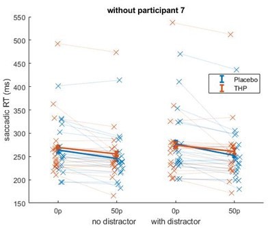
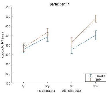
(a) Trial structure for a high incentive trial with a salient distractor. After fixation on the pink starting circle, the incentive cue plays, and after a short fixation wait the preparation cue is given which is the fixation cross turning white. 1500 ms later, one circle dims, which is the target, and on 50% of trials the other circle brightens (salient distractor). Feedback is given when participants saccade to the target, based on their speed. Timings are given below each screen. (b) Eye position as a function of time for a selection of saccades. Saccade reaction time (RT) is the time at which the saccade begins, peak velocity is the maximal speed during the movement (steepest slope here), and amplitude is the distance to the saccade endpoint. (c) Plotting peak velocity against amplitude (sample data) shows the main sequence effect (dashed lines) where larger saccades have higher velocity. We regressed velocity on amplitude separately within each drug session (to control for potential drug effects on amplitude, velocity, or the main sequence), giving residual peak velocity as our measure of vigour (solid vertical lines). (d) Mean peak residual velocity for each condition (20 participants, 18585 trials). Incentives increased velocity (single-trial linear mixed-effects regression; β=0.1266, p<0.0001; see Table 1 for full statistics), distractors decreased it (β=–0.0158, p=0.0294), and THP reduced the invigoration by incentives (β=–0.0216, p=0.0030). This interaction was significant only for the no-distractor trials. Crosses show individual participant means for each condition, and error bars show within-subject SEM. (e) Mean saccadic RT for each condition (log RT was analysed, raw values plotted here). High incentives decreased RT (β=–0.0767, p<0.0001), distractors slowed RT (β=0.0358, p<0.0001), and THP reduced the effect of incentive on RT (β=0.0218, p=0.0002) – which was driven by trials with distractors present. Crosses show individual participant means for each condition.
-
Figure 1—source code 1
Matlab code to produce Figure 1c–e (see GitHub repo for additional required functions).
- https://cdn.elifesciences.org/articles/98922/elife-98922-fig1-code1-v1.zip
-
Figure 1—source data 1
mat file with data to produce Figure 1c–e.
- https://cdn.elifesciences.org/articles/98922/elife-98922-fig1-data1-v1.zip
Figure 1—figure supplement 1
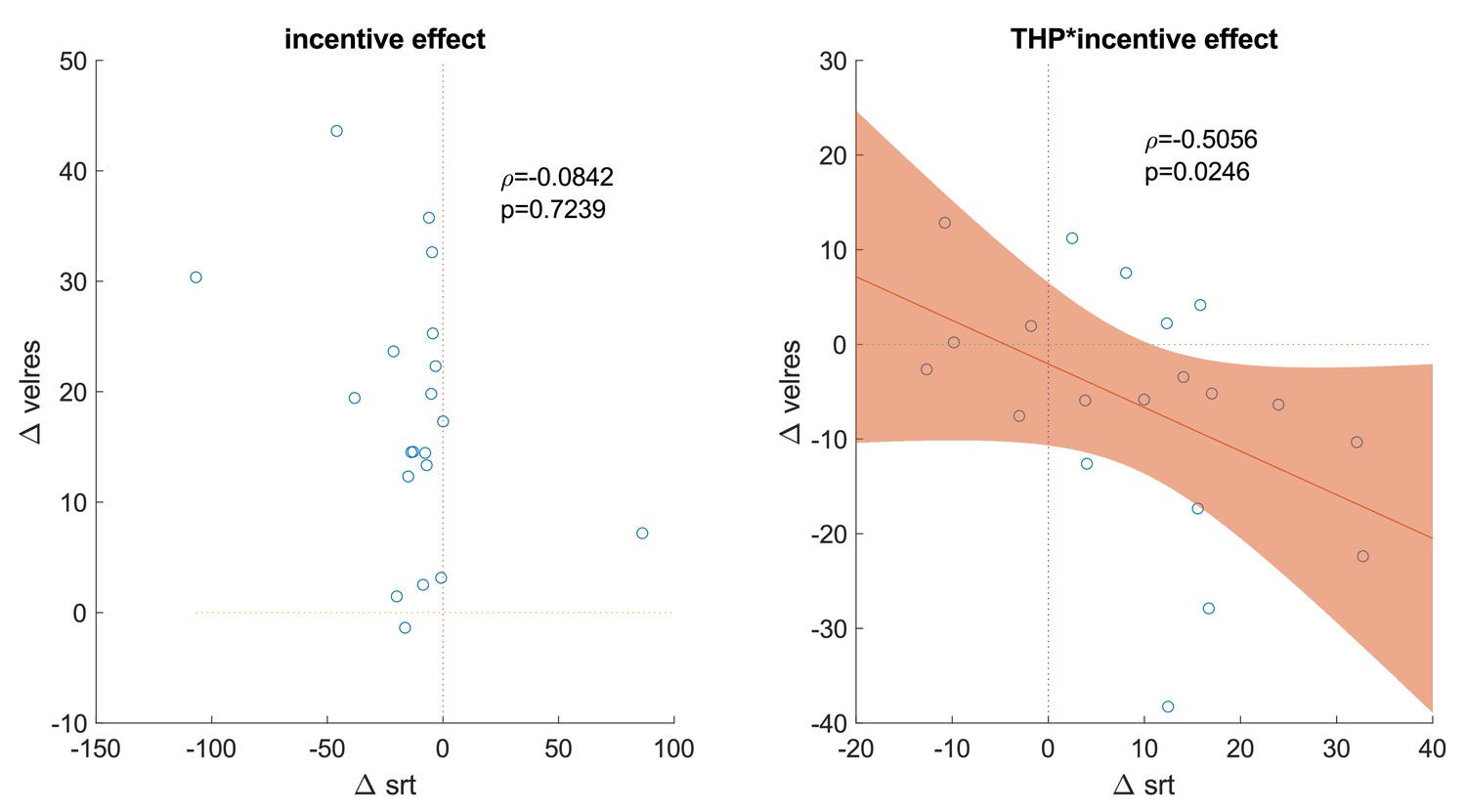
Incentive effects are uncorrelated between saccade reaction times (RT) and velocity, but the THP*incentive interactions are correlated.
The correlation is negative as RT is inverse to response speed, meaning in both variables the drug is reducing the incentive speeding effect. Each dot shows one participant’s mean (20 participants), the line is the linear correlation, the shading shows the 95% confidence interval of the slope, and the text shows the Spearman’s correlation and p-value. (a) Incentive effect is measured as the mean difference in RT and velocity between 50p and 0p conditions, averaged across drug and distractor factors. (b) THP*incentive effect is measured as the mean difference between incentive effects for the drug and placebo conditions, averaged across the distractor levels.
-
Figure 1—figure supplement 1—source code 1
Matlab code to produce Figure 1—figure supplement 1.
- https://cdn.elifesciences.org/articles/98922/elife-98922-fig1-figsupp1-code1-v1.zip
Figure 2 with 1 supplement

Muscarinic blockade increases the pull from salient distractors.
(a) Sample saccades showing fixation at the bottom left circle, the target on the right, and the distractor on the top. Distractor pull is the angle of the eye when it leaves the fixation circle, relative to a straight line from the fixation to target circle (positive values reflect angles towards the distractor, zero is flat, negative reflects repulsion). (b) Mean distractor pulls for low and high incentives when the salient distractor is and is not present (crosses show individual participant means per condition, error-bars are within-subject SEM; 20 participants, 18585 trials). Distractor pull was negative (i.e. below the horizontal line in panel a) reflecting repulsion from the distractor when it did not light up. However, when the distractor did light up, distractor pull was positive (single-trial linear mixed-effects regression; β=0.2446, p<0.0001), reflecting a bias towards it, and this bias was greater on trihexyphenidyl (THP) than placebo (distractor*THP interaction: β=0.0226, p=0.0012; full statistics are given in Table 1). (c) Mean kernel-smoothed density of distractor pulls for all trials with a distractor (averaged across all other conditions) with shading showing the within-subject standard errors. There is a smaller peak centred on the distractor’s orientation (grey dashed line and circle). Negative distractor pulls show the repulsive bias away from the distractor location. (d) Mean kernel-smoothed densities showing the effects of incentive (i.e. 50p – 0p) and THP (i.e. THP – incentive) for all ‘with distractor’ trials. Cluster-based permutation testing showed that THP reduced the number of trials biased around –30° (p<0.05), indicating reduced repulsive bias when muscarinic receptors are antagonised.
-
Figure 2—source code 1
Matlab code to produce Figure 2b–d (see GitHub repo for additional required functions).
- https://cdn.elifesciences.org/articles/98922/elife-98922-fig2-code1-v1.zip
-
Figure 2—source data 1
mat file with data for Figure 2b–d.
- https://cdn.elifesciences.org/articles/98922/elife-98922-fig2-data1-v1.zip
Figure 2—figure supplement 1
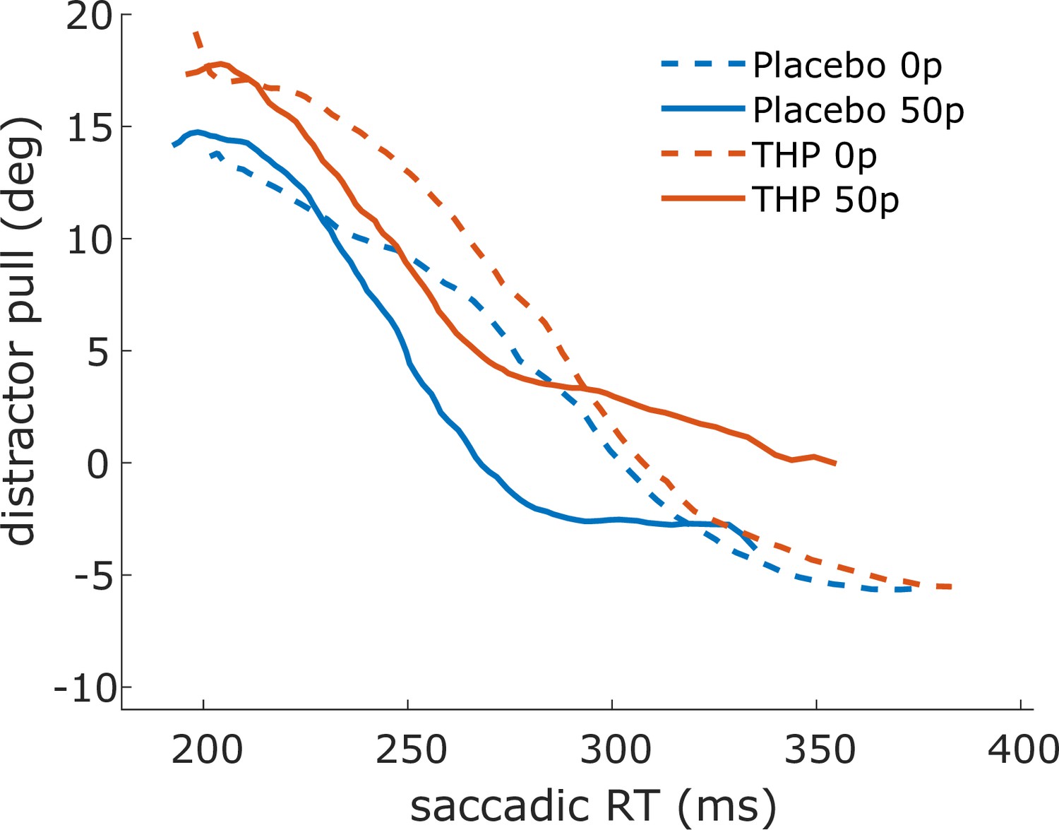
Distractor pull as a function of reaction time (RT).
For all trials with a distractor present, after binning RT into 80 percentile windows for each subject (N=20) and condition, and plotting mean distractor pull angle for each bin. Distractor pull was greatest for quickest saccades, and incentives sped responses (solid lines shifted leftwards), while trihexyphenidyl (THP) increased distraction (orange lines shifted upwards) and slowed RT (small rightwards shift). This means that for a given speed, distraction was lessened by incentives and increased by THP.
-
Figure 2—figure supplement 1—source code 1
Matlab file to produce Figure 2—figure supplement 1.
- https://cdn.elifesciences.org/articles/98922/elife-98922-fig2-figsupp1-code1-v1.zip
Figure 3 with 2 supplements
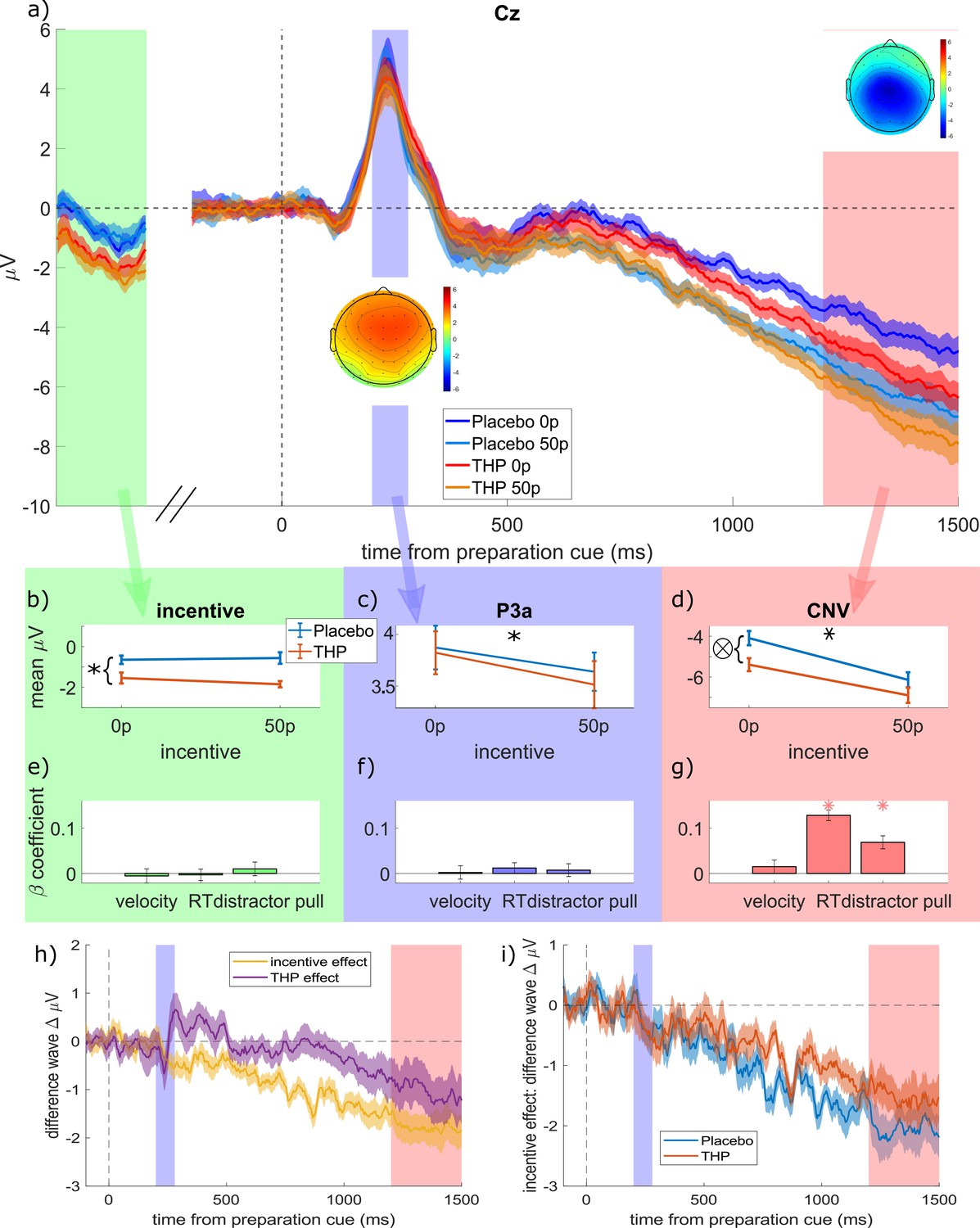
Mean event-related potentials (ERPs) to the preparation cue.
(a) Grand-average ERPs in electrode Cz split for the four conditions (low and high incentive, placebo and trihexyphenidyl [THP]; 20 participants, within-subject SEM error-bars). The three time-windows are highlighted in different colours, and correspond to the columns of panels below, with topographies of the mean amplitude within each window superimposed. The ‘incentive’ window is a non-contiguous window of 900–1100 ms after the incentive cue, just before the preparation cue appears, which contains the late negative potential after the incentive cue. (b–d) The mean voltages within each time-window for the different incentive and drug conditions (individual participants’ data are shown in Figure 3—figure supplement 1, and full statistics are given in Table 2). (b) Late ERP to the incentive cue (900:1100 ms at Cz) was more negative when on THP than placebo (single-trial linear mixed-effects regression with 16627 trials; β=–0.0597, p<0.0001), but it was not affected by incentive (p>0.05). (c) Mean P3a (200:280 ms after the preparation cue) is decreased by high incentives (β=–0.0187, p=0.0142) but unaffected by THP (p>0.1, note the different y-axis scale to b and d). (d) The contingent negative variation (CNV) (1200:1500 ms after the preparation cue) is strengthened (more negative) by incentives (β=–0.0928, p<0.0001) and THP (β=–0.0502, p<0.0001), with a weak interaction (β=0.0172, p=0.0213) as THP slightly reduces the incentive effect (flatter slope for the orange line; and THP lines are closer than placebo lines in panel a). (e–g) The beta-coefficients from regressing each component against each behavioural variable, with stars representing significant associations (p<0.0056; Bonferroni-corrected for nine comparisons, error bars are 95% CI). (h) Difference waves showing the effects of incentive (50p – 0p, averaged over other factors) and THP (THP – placebo, averaged over other factors). Incentive starts decreasing (i.e. strengthening) the CNV early (during the P3a window), while the THP effect starts around 900 ms after the preparation cue. (i) Difference waves showing incentive effects within each drug condition separately. Incentives strengthen the CNV for both conditions, with the effect growing more slowly for the THP condition, reflecting the THP*incentive interaction reported in the main text.
-
Figure 3—source code 1
Matlab code to produce figure panels (see GitHub repo for additional required functions).
- https://cdn.elifesciences.org/articles/98922/elife-98922-fig3-code1-v1.zip
-
Figure 3—source data 1
mat file with data to produce figure panels, including Figure 3—figure supplement 1.
- https://cdn.elifesciences.org/articles/98922/elife-98922-fig3-data1-v1.zip
-
Figure 3—source data 2
Linear mixed-effects single-trial regression outputs for the effect of pre-preparation cue activity, P3a, and contingent negative variation (CNV) on each behavioural measure.
Pre-preparation cue activity and P3a did not predict any behavioural measure, while CNV predicted reaction times (RT) and distractor pull (Bonferroni-corrected threshold: α=0.0056). The regression formula controlled for all factors and their interactions, and a random effect of participant: ‘ERP ~ 1 + behaviour + incentive * distractor * THP + (1 | participant)’. Significant effects are shown in bold italics.
- https://cdn.elifesciences.org/articles/98922/elife-98922-fig3-data2-v1.zip
Figure 3—figure supplement 1
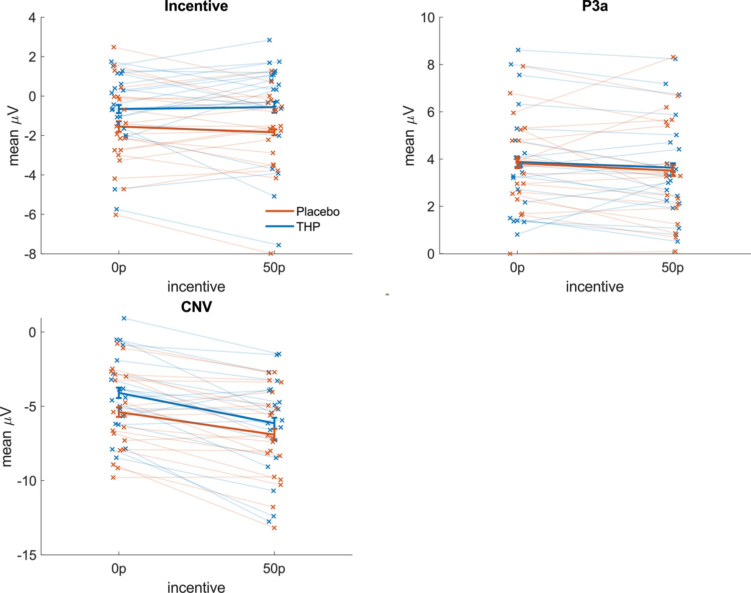
Mean individual participants’ event-related potential (ERP) component voltages for each time-window.
The means for each individual person (N=20) are superimposed on top. These figures can be created using Figure 3—source data 1.
Figure 3—figure supplement 2
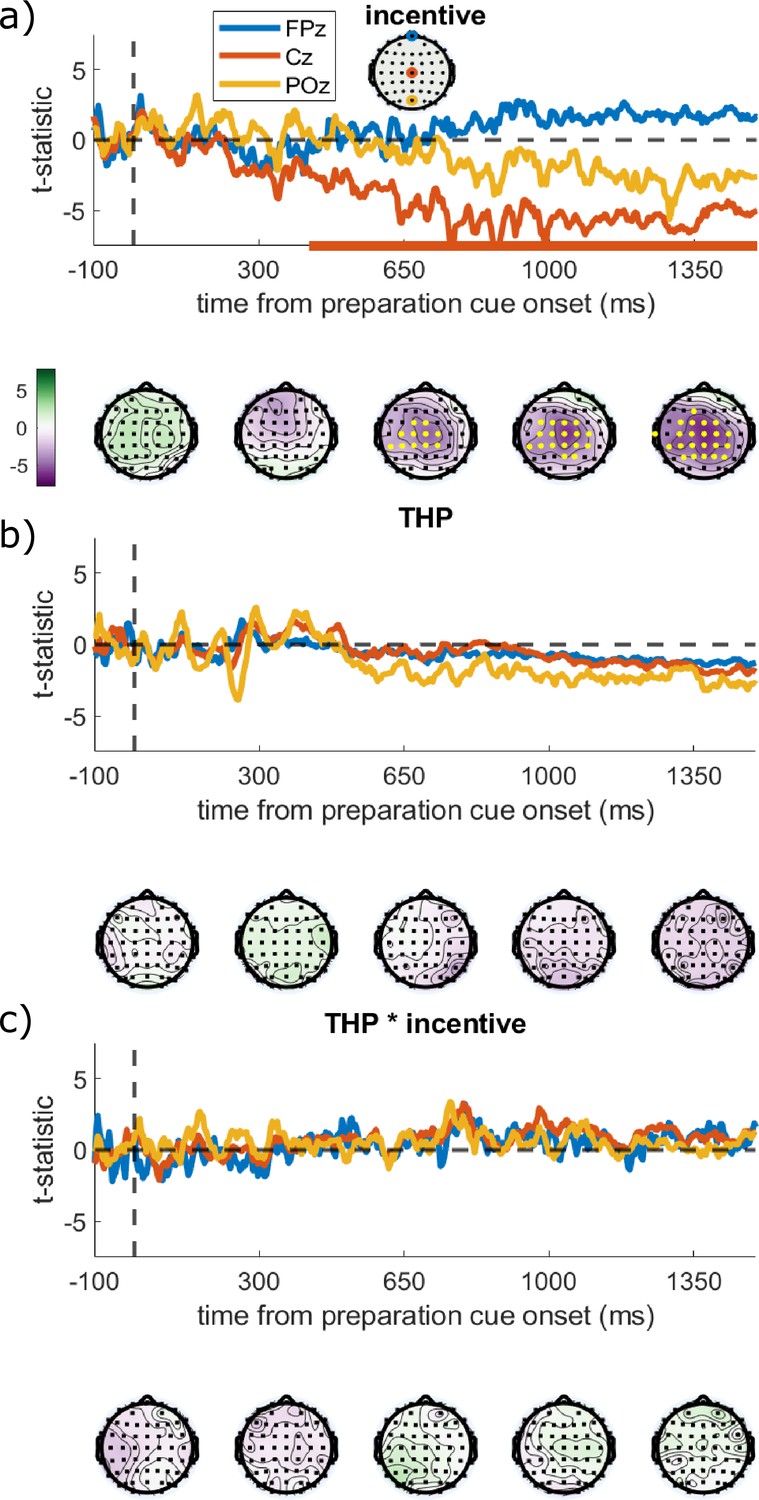
Testing for effects of incentives, trihexyphenidyl (THP), or THP*incentives across all electrodes and time-points.
We used difference waves, and difference-of-difference waves for the interaction, with cluster-based permutation testing (20 participants, 2500 iterations, family-wise error rate [FWER] = 0.05; DMGroppe Mass Univariate toolbox; Groppe et al., 2011). (a) t-Statistics for the incentive difference wave (i.e. 50p – 0p, averaged across other factors) for three selected channels, with the solid bar at the bottom showing significant clusters (FWER = 0.05). The topographies below show the t-statistics for all channels at the times written on the x-axis, with the yellow dots representing electrodes in significant clusters. Higher incentives lead to more negative voltages centro-posteriorly from about 400 ms after the preparation cue began, and this increases over the epoch. (b) t-Statistics for the drug difference wave (THP – placebo) shows no significant clusters at any channels or time-points, suggesting that THP did not change the voltage overall. (c) Difference of difference waves showing the THP*incentive interaction ((drug 50p – 0p) – (placebo 50p – 0p)) also shows no cluster of significant difference.
-
Figure 3—figure supplement 2—source data 1
mat file with data to produce Figure 3—figure supplement 2.
- https://cdn.elifesciences.org/articles/98922/elife-98922-fig3-figsupp2-data1-v1.zip
-
Figure 3—figure supplement 2—source code 1
Matlab file to produce Figure 3—figure supplement 2.
- https://cdn.elifesciences.org/articles/98922/elife-98922-fig3-figsupp2-code1-v1.zip
Figure 4 with 2 supplements
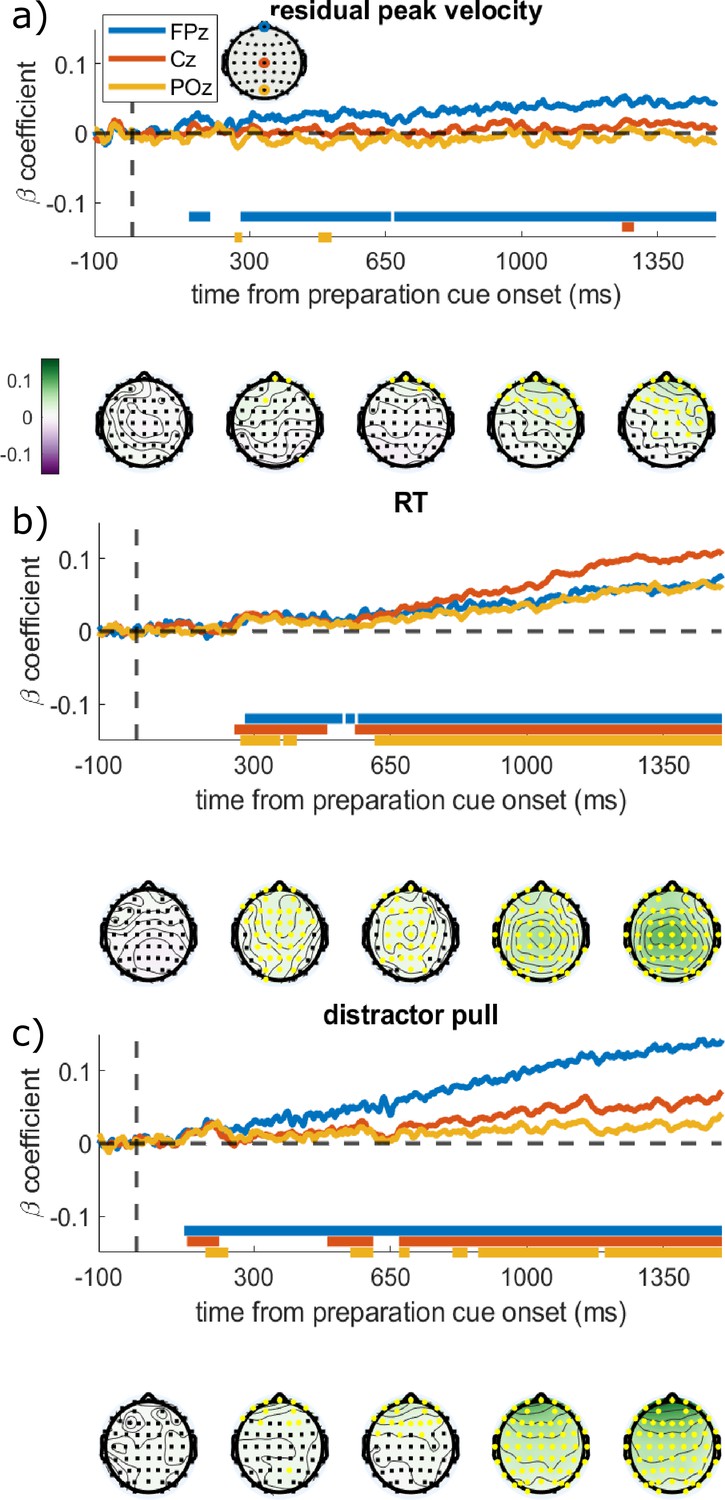
Regression coefficients from regressing each electrode and time-point against the different behavioural variables.
The time series show the regression coefficients for three chosen electrodes, with the solid bars at the bottom showing significant clusters for those electrodes (family-wise error rate [FWER] = 0.05; 20 participants, 16627 trials). Topographies are shown below the graph at the times written on the x-axis, with the colours showing the regression coefficient and yellow electrodes showing significant clusters. (a) Residual velocity is predicted by voltage in the frontal electrodes briefly from 150:190 ms after preparation cue, and then again from 280 ms onwards, and gradually spreads backwards. (b) Reaction time (RT) is predicted by almost all electrodes from 250 ms onwards, and is strongest centrally. (c) Distractor pull is predicted by frontal electrodes from 120 ms and this grows stronger over time, the central and posterior electrodes have a brief cluster around 180 ms but only become consistently associated from 650 ms.
-
Figure 4—source code 1
Matlab file to produce Figure 4.
- https://cdn.elifesciences.org/articles/98922/elife-98922-fig4-code1-v1.zip
-
Figure 4—source data 1
mat file with data to produce Figure 4.
- https://cdn.elifesciences.org/articles/98922/elife-98922-fig4-data1-v1.zip
Figure 4—figure supplement 1
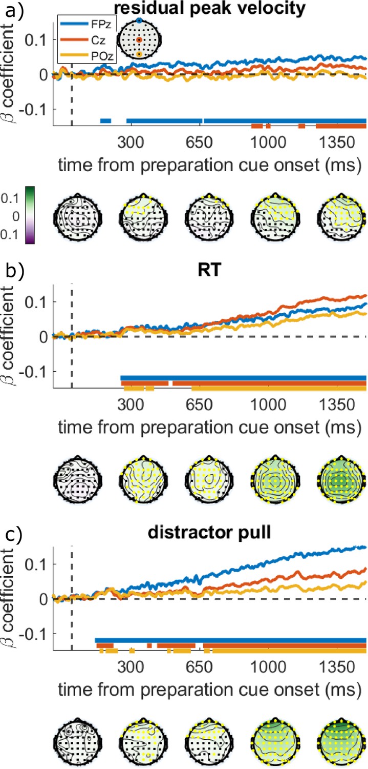
Covariate-controlled regression coefficients from regressing each electrode and time-point against the different behavioural variables.
The association between the electroencephalography (EEG) signals and each behavioural measure remained after accounting for the other two measures, with a very similar pattern to the main results (Figure 4). The time series show the regression coefficients for three chosen electrodes, with the solid bars at the bottom showing significant clusters for those electrodes (family-wise error rate [FWER] = 0.05; 20 participants). Topographies are shown below the graph at the times written on the x-axis, with the colours showing the regression coefficient and yellow electrodes showing significant clusters. (a) Residual velocity is predicted by voltage in the frontal electrodes briefly from 150:190 ms after preparation cue, and then again from 280 ms onwards, and gradually spreads backwards. (b) Reaction time (RT) is predicted by almost all electrodes from 250 ms onwards, and is strongest centrally. (c) Distractor pull is predicted by frontal electrodes from 120 ms and this grows stronger over time, the central and posterior electrodes have a brief cluster around 180 ms but only become consistently associated from 650 ms.
-
Figure 4—figure supplement 1—source data 1
mat file with data to produce Figure 4—figure supplement 1.
This can be used with the Matlab file from Figure 4—source code 1.
- https://cdn.elifesciences.org/articles/98922/elife-98922-fig4-figsupp1-data1-v1.zip
Figure 4—figure supplement 2
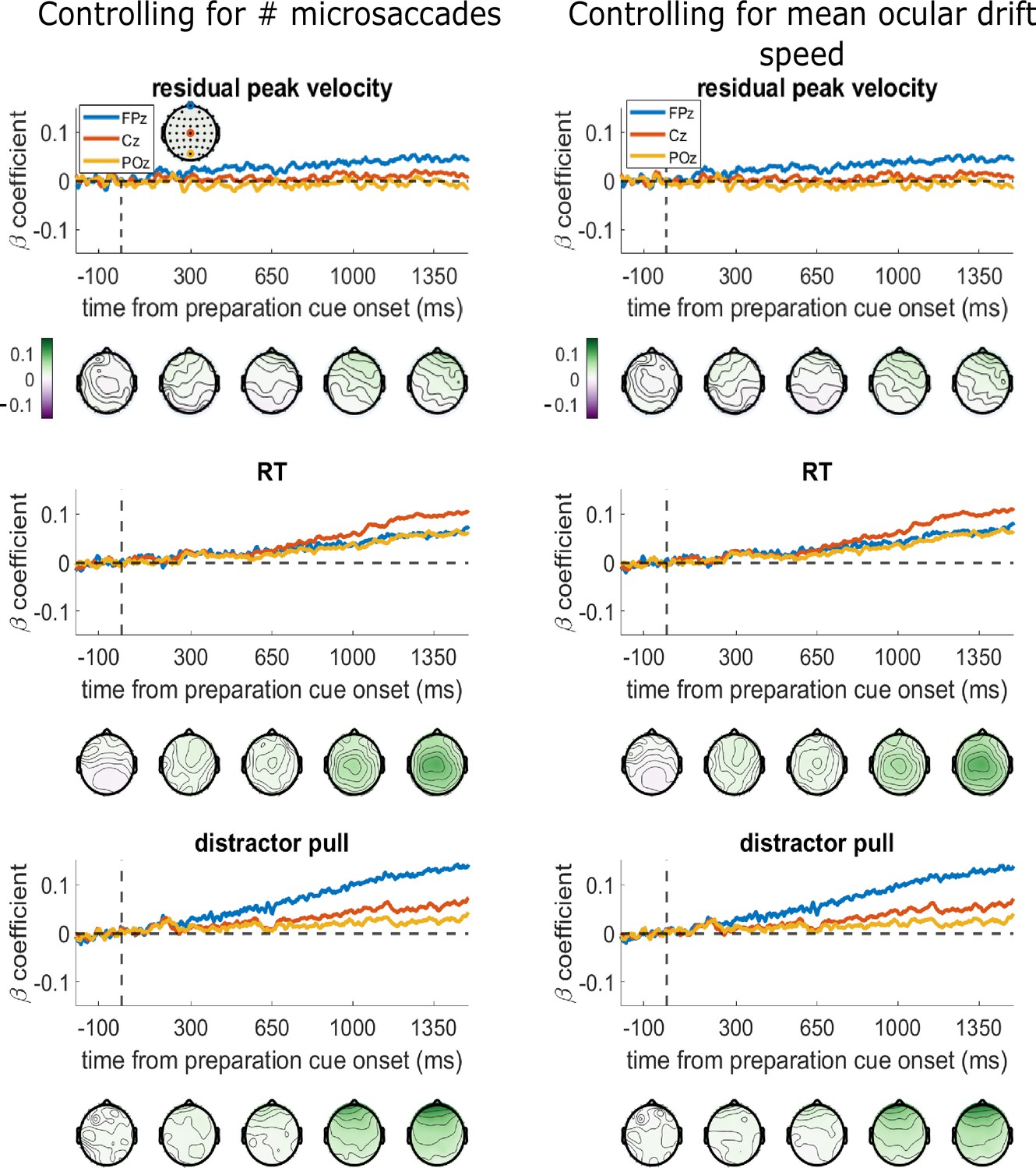
Regression analyses are relatively unchanged when controlling for eye movements.
We included either the number of microsaccades (left), or the mean ocular drift speed (right) during the entire preparation period, as covariates in the regression model. (We did not do the permutation testing for this control analysis, due to time constraints.) The beta-coefficients are almost unchanged from the analyses presented in Figure 4, either in the time-course of the selected channels or in the topographies.
-
Figure 4—figure supplement 2—source data 1
mat file with data to produce Figure 4—figure supplement 2.
This can be used with the Matlab file from Figure 4—source code 1.
- https://cdn.elifesciences.org/articles/98922/elife-98922-fig4-figsupp2-data1-v1.zip
Figure 5
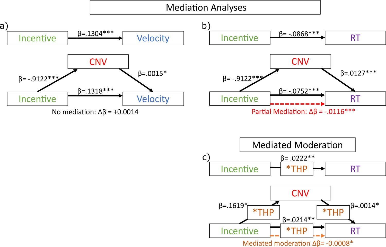
Mediation analyses of late contingent negative variation (CNV) amplitude on residual velocity and reaction times (RT).
Black lines show significant associations, with single-trial regression coefficients (20 participants, 16627 trials), and significance indicated by the text, dashed red lines show significant mediations (permutation testing), and dashed orange lines show significant mediated moderations (permutation testing). (a) There was no mediation of the incentive effect on residual velocity by the mean CNV (1200:1500 ms). (b) However, CNV does partially mediate the effect of incentive on saccadic RT (dashed red line shows the indirect effect, which is the partial mediation). (c) Mediated moderation analysis: CNV mediated the moderation of trihexyphenidyl (THP) on the incentive effect.
-
Figure 5—source data 1
mat file with the full mediation analysis output for the residual velocity analysis.
- https://cdn.elifesciences.org/articles/98922/elife-98922-fig5-data1-v1.zip
-
Figure 5—source data 2
mat file with the full mediation analysis output for the saccadic reaction time (RT) analysis.
- https://cdn.elifesciences.org/articles/98922/elife-98922-fig5-data2-v1.zip
Author response image 1

Difference in beta-coefficients when eye-movement covariates are included.
This is the difference from the beta-coefficients shown in Figure 4, please note the smaller y-axis limits.
Author response image 2

Controlling for change in eye-position at each time-point does not change the regression results.
Left column shows the beta-coefficients between the variable and EEG voltage, and the right column shows the difference from the main results in Figure 4 (note the smaller y-axis limits for the right-hand column).
Author response image 3
Author response image 4
Tables
Table 1
Linear mixed-effects single-trial regression outputs for behavioural variables.
Each model included a random effect of participant (20 participants, 18585 trials), along with all lower-order interactions and main effects: ‘behaviour ~ 1 + incentive * distractor * THP + (1 | participant)’. RT was log-transformed for this analysis. Significant effects are shown in bold italics.
| Measure | Term | β | CI | SE | t | p |
|---|---|---|---|---|---|---|
| Residual velocity (df = 1, 18,577) | Incentive | 0.1266 | 0.1123, 0.1408 | 0.0073 | 17.4001 | <0.0001 |
| Distractor | –0.0158 | −0.0301,–0.0016 | 0.0073 | –2.1786 | 0.0294 | |
| THP | –0.0001 | –0.0144, 0.0141 | 0.0073 | –0.0153 | 0.9878 | |
| Incentive * distractor | –0.0067 | 0.0201, 0.0076 | 0.0073 | –0.9143 | 0.3605 | |
| Incentive * THP | –0.0216 | −0.0358,–0.0073 | 0.0073 | –2.9678 | 0.0030 | |
| Distractor * THP | 0.0023 | –0.0120, 0.0165 | 0.0073 | 0.3152 | 0.7526 | |
| Incentive * distractor * THP | 0.0052 | –0.0091, 0.0195 | 0.0073 | 0.7158 | 0.4741 | |
| Saccade RT (df = 1, 18,577) | Incentive | –0.0767 | −0.0884,–0.0651 | 0.0059 | –12.9162 | <0.0001 |
| Distractor | 0.0348 | 0.0231, 0.0464 | 0.0059 | 5.8549 | <0.0001 | |
| THP | 0.0244 | 0.0127, 0.0360 | 0.0059 | 4.1010 | <0.0001 | |
| Incentive * distractor | –0.0035 | –0.0151, 0.0082 | 0.0059 | –0.5826 | 0.5601 | |
| Incentive * THP | 0.0218 | 0.0102, 0.0335 | 0.0059 | 3.6723 | 0.0002 | |
| Distractor * THP | –0.0117 | −0.0233,–0.0001 | 0.0059 | –1.9689 | 0.0490 | |
| Incentive * distractor * THP | 0.0076 | –0.0041, 0.0192 | 0.0059 | 1.2714 | 0.2036 | |
| Distractor pull (df = 1, 18,577) | Incentive | 0.0023 | –0.0114, 0.0160 | 0.0070 | 0.3261 | 0.7444 |
| Distractor | 0.2446 | 0.2309, 0.2583 | 0.0070 | 35.0416 | <0.0001 | |
| THP | 0.0283 | 0.0146, 0.0420 | 0.0070 | 4.0570 | <0.0001 | |
| Incentive * distractor | 0.0028 | –0.0109, 0.0165 | 0.0070 | 0.3982 | 0.6905 | |
| Incentive * THP | 0.0030 | –0.0107, 0.0167 | 0.0070 | 0.4340 | 0.6643 | |
| Distractor * THP | 0.0226 | 0.0089, 0.0363 | 0.0070 | 3.2348 | 0.0012 | |
| Incentive * distractor * THP | –0.0039 | –0.0177, 0.0098 | 0.0070 | –0.5631 | 0.5734 |
Table 2
Linear mixed-effects single-trial regression outputs for P3a and contingent negative variation (CNV).
Significant effects are shown in bold italics. Each model also included a random effect of participant, along with all lower-order interactions and main effects: ‘ERP ~ 1 + incentive * distractor * THP + (1 | participant)’. There were 20 participants and 16627 trials in total.
| Measure | Term | β | CI | SE | t | p |
|---|---|---|---|---|---|---|
| P3a (df = 1, 16,619) | Incentive | –0.0186 | −0.0335,–0.0037 | 0.0076 | –2.4509 | 0.0143 |
| Distractor | –0.0088 | –0.0237, 0.0061 | 0.0076 | –1.1572 | 0.2472 | |
| THP | 0.0004 | –0.0153, 0.0145 | 0.0076 | 0.0490 | 0.9610 | |
| Incentive * distractor | –0.0042 | –0.0191, 0.0107 | 0.0076 | –0.5557 | 0.5785 | |
| Incentive * THP | –0.0002 | –0.0169, 0.0129 | 0.0076 | –0.2656 | 0.7906 | |
| Distractor * THP | –0.0095 | –0.0244, 0.0054 | 0.0076 | –1.2467 | 0.2125 | |
| Incentive * distractor * THP | 0.0054 | –0.0095, 0.0203 | 0.0076 | 0.7118 | 0.4766 | |
| CNV (df = 1, 16,619) | Incentive | –0.0917 | −0.0106,–0.0771 | 0.0075 | –12.258 | <0.0001 |
| Distractor | –0.0032 | –0.0178, 0.0115 | 0.0075 | –0.4278 | 0.6688 | |
| THP | –0.0512 | −0.0659,–0.0365 | 0.0075 | –6.8409 | <0.0001 | |
| Incentive * distractor | –0.0002 | –0.0149, 0.0144 | 0.0075 | –0.0301 | 0.9760 | |
| Incentive * THP | 0.0165 | 0.0018, 0.0311 | 0.0075 | 2.2036 | 0.0276 | |
| Distractor * THP | –0.0042 | –0.0188, 0.0105 | 0.0075 | –0.5560 | 0.5762 | |
| Incentive * distractor * THP | –0.0037 | –0.0184, 0.0109 | 0.0075 | –0.4974 | 0.6189 | |
| Pre-preparation cue (df = 1, 15,879) | Incentive | –0.0006 | –0.0158, 0.0147 | 0.0078 | –0.0712 | 0.9430 |
| Distractor | 0.0064 | –0.0089, 0.0216 | 0.0078 | 0.8186 | 0.4130 | |
| THP | –0.0597 | −0.0751,–0.0443 | 0.0078 | –7.6126 | <0.0001 | |
| Incentive * distractor | –0.0039 | –0.0191, 0.0114 | 0.0078 | –0.4959 | 0.6200 | |
| Incentive * THP | –0.0127 | –0.0279, 0.0026 | 0.0078 | –1.6256 | 0.1041 | |
| Distractor * THP | –0.0015 | –0.0168, 0.0137 | 0.0078 | –0.1963 | 0.8444 | |
| Incentive * distractor * THP | –0.0030 | –0.0183, 0.0123 | 0.0078 | –0.3843 | 0.7008 |
Additional files
Download links
A two-part list of links to download the article, or parts of the article, in various formats.
Downloads (link to download the article as PDF)
Open citations (links to open the citations from this article in various online reference manager services)
Cite this article (links to download the citations from this article in formats compatible with various reference manager tools)
Muscarinic receptors mediate motivation via preparatory neural activity in humans
eLife 13:RP98922.
https://doi.org/10.7554/eLife.98922.3


