Figures and data in Untangling stability and gain modulation in cortical circuits with multiple interneuron classes

Figures
Tables
Additional files

8 figures, 1 table and 1 additional file

Figures

Figure 1

Download asset Open asset

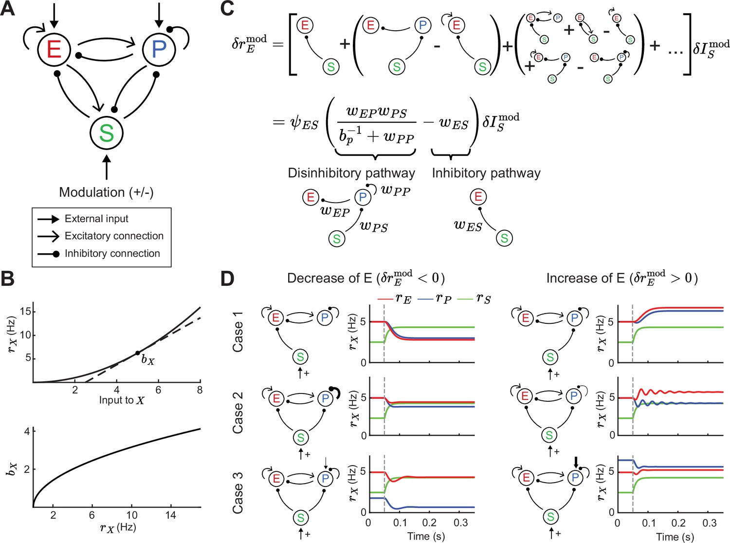
Tradeoff between two inhibitory motifs in the excitatory (E) – parvalbumin (PV) – somatostatin (SOM) cortical circuit.

(A) Sketch of the full E – PV – SOM network model. A positive or negative modulatory input is applied to the SOM neurons. (B) Transfer function (top) and population gain $b_{X}$ (bottom) for neuron population $X = {E, P, S}$ (see Equation 4). (C) Top: Relation between modulation of input to the SOM population $δ I_{S}^{m o d}$ and changes in E rates $δ r_{E}^{m o d}$ when summing over all possible paths (see Equation 10). Bottom: After summing over all paths. Sketches visualize the tradeoff between the inhibitory and disinhibitory pathways (see Equation 15). (D) Positive SOM modulation at 0.05 s (gray dashed line) decrease (left, $δ r_{E}^{m o d} < 0$ ) or increase (right, $δ r_{E}^{m o d} > 0$ ) the E rate $r_{E}$ (red line). Case 1: Add connection of SOM → E or SOM → PV population. Case 2: Change strength of self-inhibition of PV population. Case 3: Change the rate of PV neurons.

Figure 2

Download asset Open asset

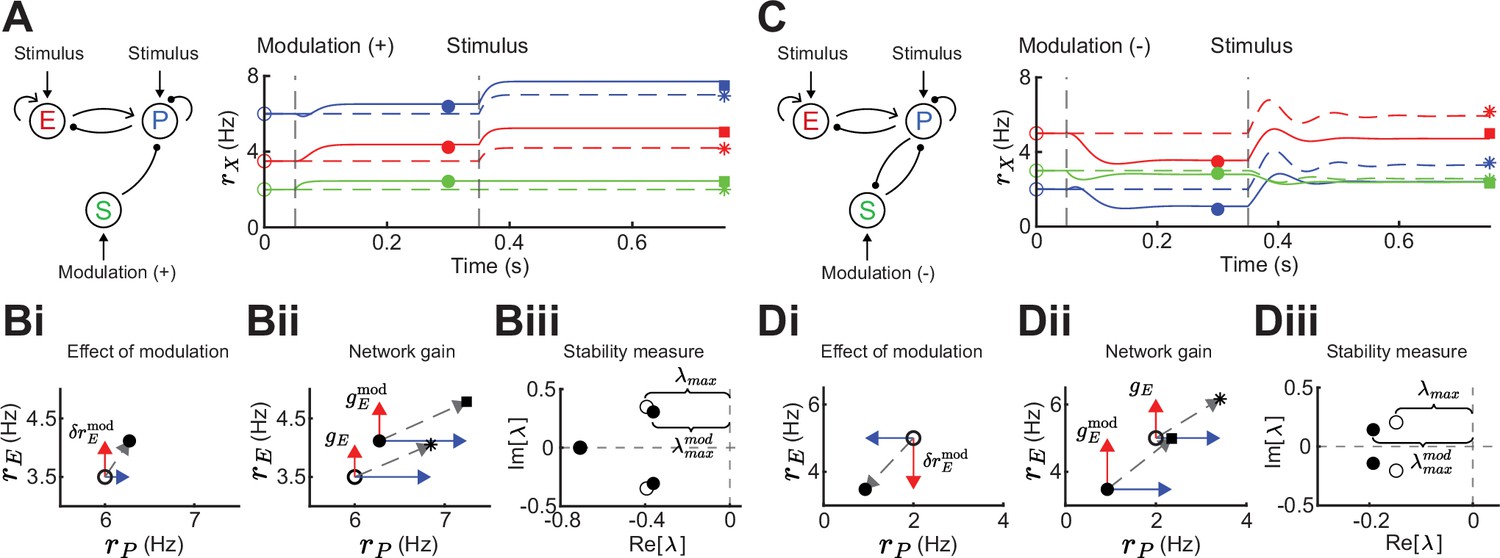
Gain and stability in excitatory (E) – parvalbumin (PV) – somatostatin (SOM) circuits.

(A) Left: Sketch of a disinhibitory network with stimulus input onto E and PV populations and positive SOM modulation. Right: Numerical E (red), PV (blue), and SOM (green) rate dynamics of the case with positive SOM modulation at 0.05 s (solid line), and the case without modulation (dashed line). Stimulus presentation at 0.35 s. Symbols indicate calculated values based on Equation 1 and Equation 2. (B) Measures to quantify the effect of SOM modulation: (i) Effect of modulation on E ( $δ r_{E}^{m o d}$ ) and PV rates, (ii) calculation of network gain with ( $g_{E}^{m o d}$ ) and without ( $g_{E}$ ) SOM modulation, $Δ g = g_{E}^{m o d} - g_{E} = 0.12$ , (**iii**) calculation of stability measure with ( $λ_{m a x}^{m o d}$ ) and without ( $λ_{m a x}$ ) SOM modulation, $Δ λ = λ_{m a x} - λ_{m a x}^{m o d} = - 0.03$ . (C) Same as A for a negative SOM modulation in a disinhibitory circuit with feedback PV → SOM. (D) Same as B for a negative SOM modulation with (ii) $Δ g = 0.35$ , and (**iii**) $Δ λ = 0.04$ (only maximum eigenvalues shown).

Figure 3

Download asset Open asset

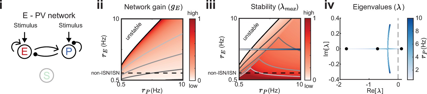
Network gain and stability in the excitatory (E) – parvalbumin (PV) network.

Network sketch (i), firing rate grid ( $r_{E}, r_{P}$ ) in the form of a heatmap for normalized network gain $g_{E}$ (ii) and normalized stability $λ_{m a x}$ (**iii**), and the eigenvalues for changing PV rates $r_{P}$ (iv) for a network without connections between the E – PV network and somatostatin (SOM). Every value in the heatmap is a fixed point of the population rate dynamics. The color denotes normalized network gain (Equation 2) or normalized stability (Figure 2Biii). Lines of constant network gain and stability are shown in gray (from dark to light gray in steps of 0.2). The black line marks where the rate dynamics become unstable. The black dashed line separates inhibition stabilized network (ISN) from non-ISN regime. Blue line in iii indicates the parameters for which the eigenvalues are shown in (iv).

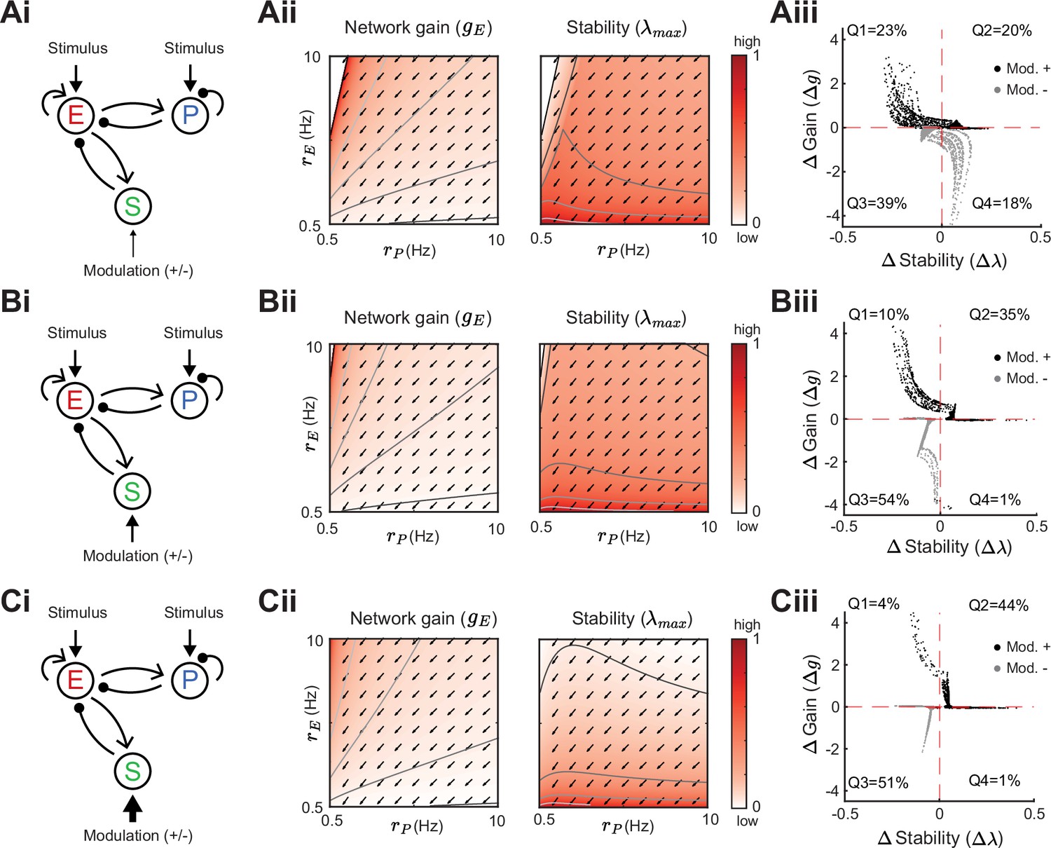
Figure 4

Download asset Open asset

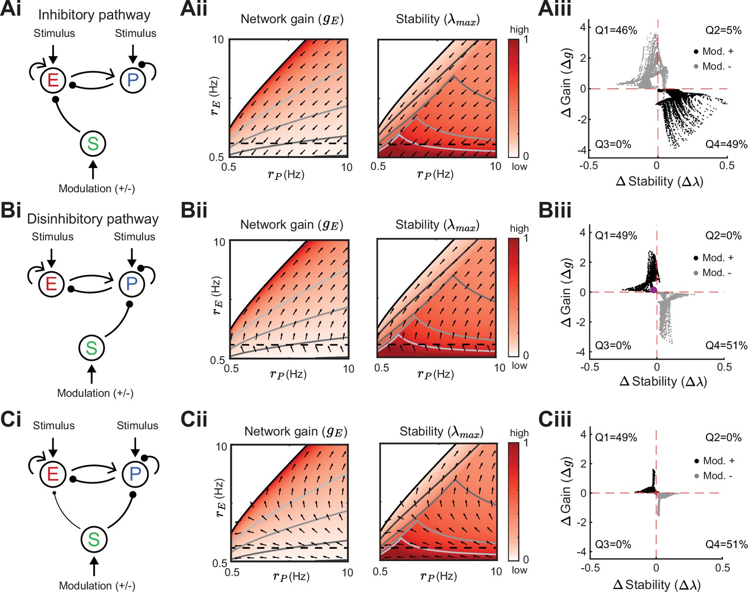
Modulation of somatostatin (SOM) neurons with feedforward SOM connectivity.

(A) Network sketch (i), firing rate grid ( $r_{E}, r_{P}$ ) in the form of a heatmap for normalized network gain and stability (ii), and modulation measures $Δ$ Gain ( $Δ g$ ) and $Δ$ Stability ( $Δ λ$ ) (iii), for a network with SOM → E connection (inhibitory pathway). The arrows indicate in which direction a fixed point of the rate dynamics is changed by a positive SOM modulation. All arrow lengths are set to the same value. The modulation measure quantifies the change in stability and gain from an initial condition in the ( $r_{E}, r_{P}$ ) grid for a positive (black dots) and negative (gray dots) SOM modulation. Q1-Q4 indicates the percent of data points in the respective quadrant (only $| Δ g | > 0.1$ and $| Δ λ | > 0.01$ are considered). (B) Same as A for a network with SOM → PV connection (disinhibitory pathway). The purple dot in Biii is the case of Figure 2A. (C) Same as A for a network with SOM → E and SOM → PV connections. SOM rate $r_{S} = 2$ Hz in all panels.

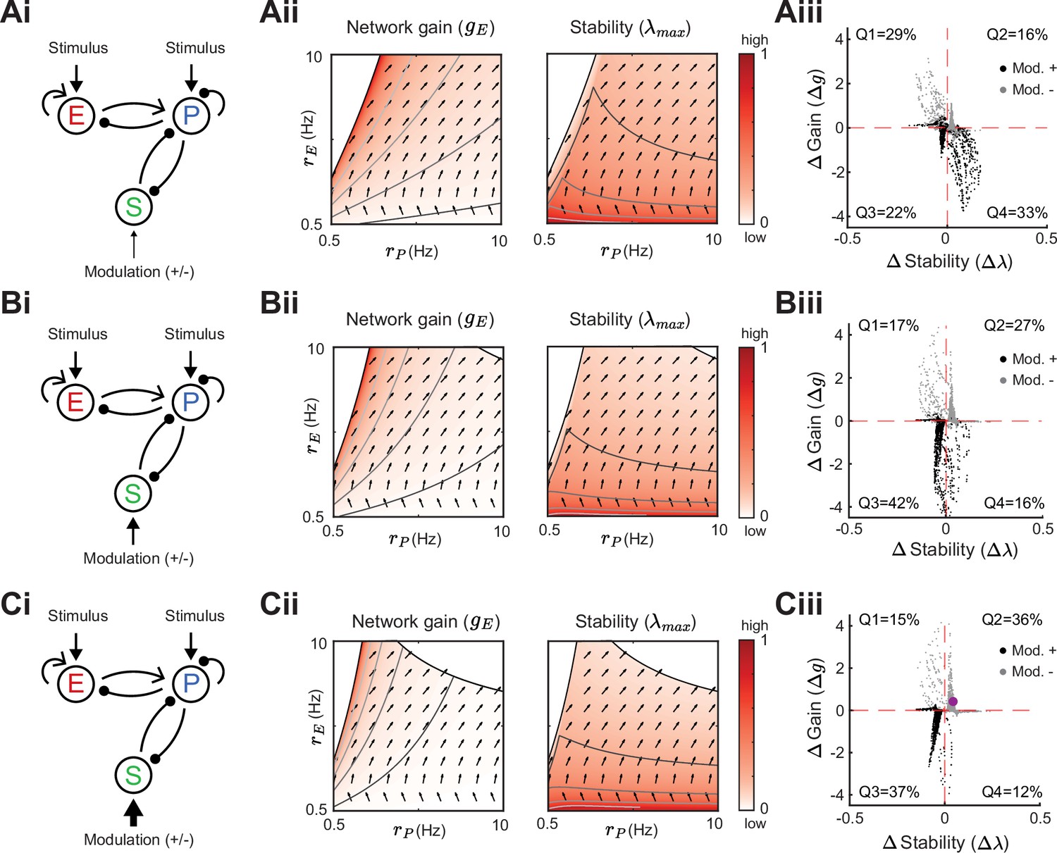
Figure 5 with 2 supplements

Download asset Open asset

Modulation of somatostatin (SOM) neurons with excitatory (E) to SOM feedback.

Heatmaps and modulation measures as defined in Figures 3 and 4 for a network with an inhibitory pathway and E → SOM feedback. Left to right: Network sketch (i), normalized network gain ( $g_{E}$ ) and stability ( $λ_{m a x}$ ) (ii), and modulation measures $Δ$ Gain ( $Δ g$ ) and $Δ$ Stability ( $Δ λ$ ) (**iii**). Top to bottom: increase of the SOM firing rate from $r_{S} = 1$ Hz (A), to $r_{S} = 2$ Hz (B), $r_{S} = 3$ Hz (C). The arrows indicate in which direction a fixed point of the rate dynamics is changed by a positive SOM modulation.

Figure 5—figure supplement 1

Download asset Open asset

Modulation of somatostatin (SOM) neurons with parvalbumin (PV) to SOM feedback.

Same as Figure 5 for a network with a disinhibitory pathway and PV → SOM feedback ( $w_{S P}$ ). Left to right: Network sketch (i), Network gain ( $g_{E}$ ) and stability (λ_max) (ii), and modulation measures Δ Gain (Δg) and Δ Stability (Δλ) (iii). Top to bottom: increase of the SOM firing rate from $r_{S} = 1$ Hz (A), to $r_{S} = 2$ Hz (B), $r_{S} = 3$ Hz (C). The purple dot corresponds to the case in Figure 2C.

Figure 5—figure supplement 2

Download asset Open asset

Percent of data points in Q1-Q4 when changing somatostatin (SOM) firing rate.

(A) Percentage of data points in Q1 (black), Q2 (orange), Q3 (green), Q4 (blue) when changing the SOM firing rate $r_{S}$ for the case of excitatory neurons (E) to SOM feedback (compare to Figure 5). (B) Same as A, for the case of parvalbumin (PV) to SOM feedback (compare to Figure 5—figure supplement 1).

Figure 6

Download asset Open asset

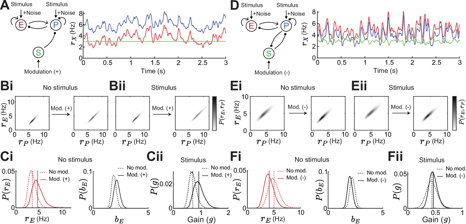
Gain and stability in noisy excitatory (E) – parvalbumin (PV) – somatostatin (SOM) circuits.

(A) Left: Sketch of a disinhibitory network with stimulus plus noise input onto E and PV populations and positive SOM modulation. Right: Numerical E (red), PV (blue), and SOM (green) rate dynamics. (B) Distribution of E and PV rates for a positive SOM modulation without (i) and with a stimulus (ii) (C) Changes in the distribution of E rates $r_{E}$ (i, left), E population gain $b_{E}$ (i, right) and network gain $g$ (ii) with vs without SOM modulation. Variance of E rates for no SOM modulation is 0.7 and with SOM modulation 1.3. (D) Same as A for a negative SOM modulation in a disinhibitory circuit with feedback PV → SOM. (E) Same as B for negative SOM modulation. Variance of E rates for no SOM modulation is 1.1 and with SOM modulation 0.8. (F) Same as C for negative SOM modulation.

Figure 7 with 1 supplement

Download asset Open asset

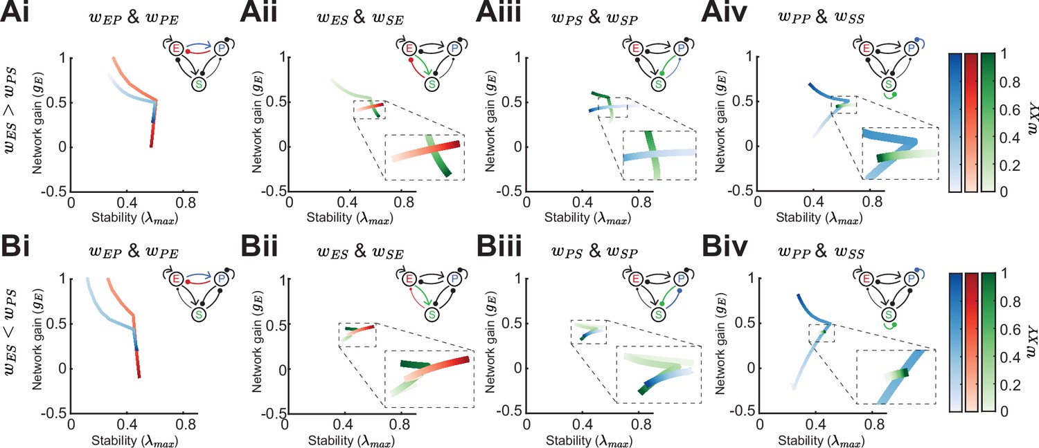
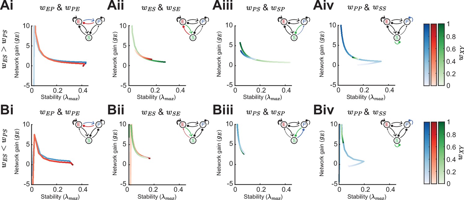
Effect of synaptic weight strength on network gain and stability.

(A) Effect of synaptic weight change on network gain ( $g_{E}$ ) and stability ( $λ_{m a x}$ ) in a network biased to inhibitory somatostatin (SOM) influence ( $w_{E S} > w_{P S}$ ). We change the strength of one weight at a time, either $w_{E P}$ or $w_{P E}$ (i), $w_{E S}$ or $w_{S E}$ (ii), $w_{P S}$ or $w_{S P}$ (iii), or $w_{P P}$ or $w_{S S}$ (iv). Colorbar indicates the weight strength, red corresponds to weights onto excitatory neurons (E) blue onto parvalbumin (PV), and green onto SOM. (B) Same as A but in a network biased to disinhibitory SOM influence ( $w_{E S} < w_{P S}$ ). The networks are in the non-inhibition stabilized network (ISN) regime ( $w_{E E}$ is weak) and all the rates are fixed $r_{E} = 3$ , $r_{P} = 5$ , $r_{S} = 0.5$ . Dashed rectangles represent zoom-in.

Figure 7—figure supplement 1

Download asset Open asset

Effect of synaptic weight strength on network gain and stability (inhibition stabilized network, ISN regime).

(A) Effect of synaptic weight change on network gain ( $g_{E}$ ) and stability ( $λ_{m a x}$ ) in a network biased to inhibitory somatostatin (SOM) influence ( $w_{E S} > w_{P S}$ ). We change the strength of one weight at a time, either $w_{E P}$ or $w_{P E}$ (i), $w_{E S}$ or $w_{S E}$ (ii), $w_{P S}$ or $w_{S P}$ (iii), or $w_{P P}$ or $w_{S S}$ (iv). Colorbar indicates the weight strength, red corresponds to weights onto excitatory neurons (E), blue onto parvalbumin (PV), and green onto SOM. (B) Same as A but in a network biased to disinhibitory SOM influence ( $w_{E S} < w_{P S}$ ). The networks are in the ISN regime ( $w_{E E}$ is strong) and all the rates are fixed, $r_{E} = 3$ , $r_{P} = 5$ . $r_{S} = 0.5$ .

Figure 8

Download asset Open asset

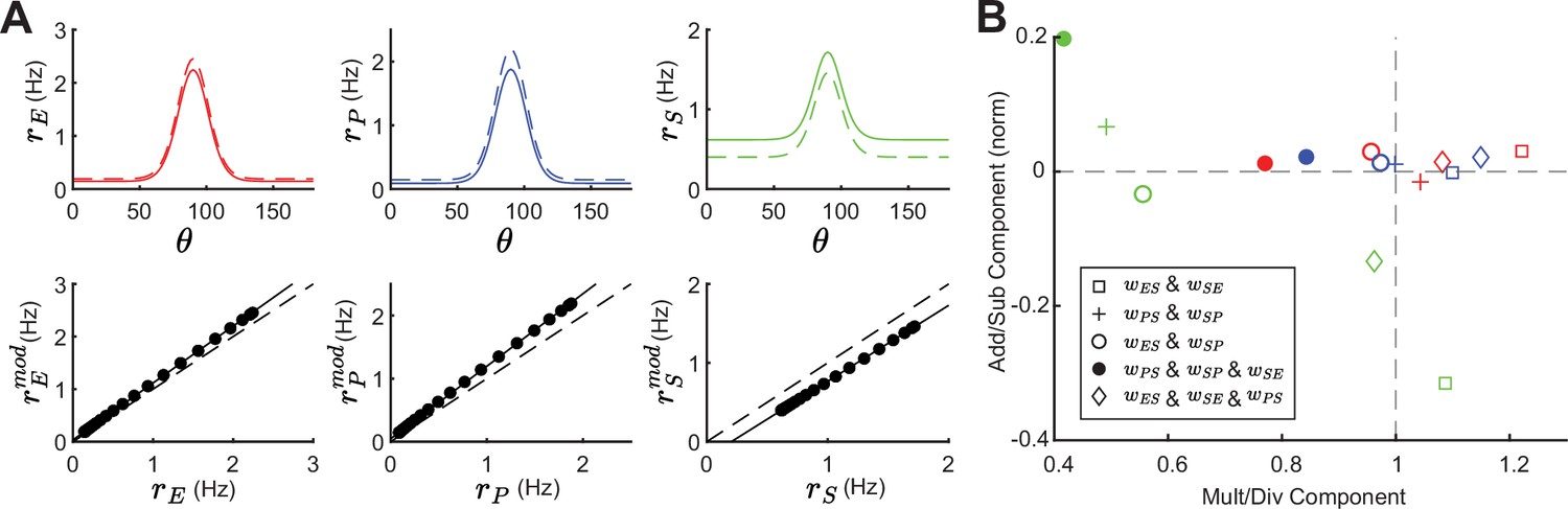
Tuning curve changes induced by somatostatin (SOM) modulation depend on network connectivity.

(A) Top: Tuning curves of excitatory (E) (red), parvalbumin (PV) (blue), and SOM (green) populations in a network with connections SOM → E and SOM → PV and a feedback connection E → SOM ( $w_{E S}, w_{P S}, w_{S E} \neq 0$ ). Solid lines represent the tuning curve before modulation and dashed lines after a negative SOM modulation. Bottom: Linear regression of unmodulated versus modulated rates (black dots: unmodulated versus modulated rate pairs, gray solid line: fit, gray dashed line: unity line). (B) Multiplicative/divisive component versus additive/subtractive component for different network connectivities. Add/sub component is normalized to the maximum rate response. Diamond case is shown in panel A.

Tables

Table 1

Weight parameters.

Figure	$w_{E E}$	$w_{E P}$	$w_{P E}$	$w_{P P}$	$w_{E S}$	$w_{P S}$	$w_{S E}$	$w_{S P}$
Figure 1C, Case 1 (left)	0.8	0.5	1	0.6	0.2	0	0	0
Figure 1C, Case 1 (right)		0.5		0.6	0	0.2
Figure 1C, Case 2 (left)		1		1	0.5	0.6
Figure 1C, Case 2 (right)				0.1
Figure 1C, Case 3				0.6
Figure 2A and B		0.5			0	0.8
Figure 2C and D						0.8		0.2
Figure 3						0		0
Figure 4A					0.8	0
Figure 4B					0	0.8
Figure 4C					0.3	0.8
Figure 5, Figure 5—figure supplement 2A					0.8	0	0.2
Figure 5—figure supplement 1					0	0.8	0	0.2
Figure 5—figure supplement 2B								0.2
Figure 6A–C								0
Figure 6D–F								0.2
Figure 8A and B, $◊$					0.5		0.5	0
Figure 8B, $◻$					0.8	0	0.5	0
Figure 8B, $+$					0	0.8	0	0.5
Figure 8B, $\circ$					0.8	0	0
Figure 8B, $∙$					0	0.8	0.5

Additional files

MDAR checklist: https://cdn.elifesciences.org/articles/99808/elife-99808-mdarchecklist1-v1.pdf
Download elife-99808-mdarchecklist1-v1.pdf

Download links

A two-part list of links to download the article, or parts of the article, in various formats.

Downloads (link to download the article as PDF)

Open citations (links to open the citations from this article in various online reference manager services)

Mendeley

Cite this article (links to download the citations from this article in formats compatible with various reference manager tools)

Hannah Bos
Christoph Miehl
Anne-Marie Michelle Oswald
Brent Doiron

(2025)

Untangling stability and gain modulation in cortical circuits with multiple interneuron classes

eLife 13:RP99808.

https://doi.org/10.7554/eLife.99808.4

Share this article

Cite this article

Tradeoff between two inhibitory motifs in the excitatory (E) – parvalbumin (PV) – somatostatin (SOM) cortical circuit.

Gain and stability in excitatory (E) – parvalbumin (PV) – somatostatin (SOM) circuits.

Network gain and stability in the excitatory (E) – parvalbumin (PV) network.

Modulation of somatostatin (SOM) neurons with feedforward SOM connectivity.

Modulation of somatostatin (SOM) neurons with excitatory (E) to SOM feedback.

Modulation of somatostatin (SOM) neurons with parvalbumin (PV) to SOM feedback.

Percent of data points in Q1-Q4 when changing somatostatin (SOM) firing rate.

Gain and stability in noisy excitatory (E) – parvalbumin (PV) – somatostatin (SOM) circuits.

Effect of synaptic weight strength on network gain and stability.

Effect of synaptic weight strength on network gain and stability (inhibition stabilized network, ISN regime).

Tuning curve changes induced by somatostatin (SOM) modulation depend on network connectivity.

Weight parameters.

MDAR checklist

Downloads (link to download the article as PDF)

Open citations (links to open the citations from this article in various online reference manager services)

Cite this article (links to download the citations from this article in formats compatible with various reference manager tools)