Aberration correction in long GRIN lens-based microendoscopes for extended field-of-view two-photon imaging in deep brain regions

Reviewer #1 (Public review):

Summary:

Sattin, Nardin, and colleagues designed and evaluated corrective microlenses that increase the useable field of view of two long (>6mm) thin (500 um diameter) GRIN lenses used in deep-tissue two-photon imaging. This paper closely follows the thread of earlier work from the same group (esp. Antonini et al, 2020; eLife), filling out the quiver of available extended-field-of-view 2P endoscopes with these longer lenses. The lenses are made by a molding process that appears practical and easy to adopt with conventional two-photon microscopes.

Simulations are used to motivate the benefits of extended field of view, demonstrating that more cells can be recorded, with less mixing of signals in extracted traces, when recorded with higher optical resolution. In vivo tests were performed in piriform cortex, which is difficult to access, especially in chronic preparations.

The design, characterization, and simulations are clear and thorough, but they do not break new ground in optical design or biological application. However, the approach shows much promise, including for applications such as miniaturized GRIN-based microscopes. Readers will largely be interested in this work for practical reasons: to apply the authors' corrected endoscopes to their own research.

Strengths:

The text is clearly written, the ex vivo analysis is thorough and well supported, and the figures are clear. The authors achieved their aims, as evidenced by the images presented, and were able to make measurements from large numbers of cells simultaneously in vivo in a difficult preparation.

The authors did a good job of addressing issues I raised in initial review, including analyses of chromaticity and the axial field of view, descriptions of manufacturing and assembly yield, explanations in the text of differences between ex vivo and in vivo imaging conditions, and basic analysis of the in vivo recordings relative to odor presentations. They have also shortened the text, reduced repetition, and better motivated their approach in the introduction.

Weaknesses:

As discussed in review and nicely simulated by the authors, the large figure error indicated by profilometry (~10 um in some cases on average) is inconsistent with the optical performance improvements observed, suggesting that those measurements are inaccurate. I see no reason to include these inaccurate measurements.

Reviewer #2 (Public review):

In this manuscript, the authors present an approach to correct GRIN lens aberrations, which primarily cause a decrease in signal-to-noise ratio (SNR), particularly in the lateral regions of the field-of-view (FOV), thereby limiting the usable FOV. The authors propose to mitigate these aberrations by designing and fabricating aspherical corrective lenses using ray trace simulations and two-photon lithography, respectively; the corrective lenses are then mounted on the back aperture of the GRIN lens.

This approach was previously demonstrated by the same lab for GRIN lenses shorter than 4.1 mm (Antonini et al., eLife, 2020). In the current work, the authors extend their method to a new class of GRIN lenses with lengths exceeding 6 mm, enabling access to deeper brain regions as most ventral region of the mouse brain. Specifically, they designed and characterized corrective lenses for GRIN lenses measuring 6.4 mm and 8.8 mm in length. Finally, they applied these corrected long micro-endoscopes to perform high-precision calcium signal recordings in the olfactory cortex.

Compared with alternative approaches using adaptive optics, the main strength of this method is that it does not require hardware or software modifications, nor does it limit the system's temporal resolution. The manuscript is well-written, the data are clearly presented, and the experiments convincingly demonstrate the advantages of the corrective lenses.

The implementation of these long corrected micro-endoscopes, demonstrated here for deep imaging in the mouse olfactory bulb, will also enable deep imaging in larger mammals such as rats or marmosets.

Comments on revisions:

The authors have clearly addressed all my comments.

Reviewer #3 (Public review):

Summary:

This work presents the development, characterization and use of new thin microendoscopes (500µm diameter) whose accessible field of view has been extended by the addition of a corrective optical element glued to the entrance face. Two microendoscopes of different lengths (6.4mm and 8.8mm) have been developed, allowing imaging of neuronal activity in brain regions >4mm deep. An alternative solution to increase the field of view could be to add an adaptive optics loop to the microscope to correct the aberrations of the GRIN lens. The solution presented in this paper does not require any modification of the optical microscope and can therefore be easily accessible to any neuroscience laboratory performing optical imaging of neuronal activity.

Strengths:

(1) The paper is generally clear and well written. The scientific approach is well structured and numerous experiments and simulations are presented to evaluate the performance of corrected microendoscopes. In particular, we can highlight several consistent and convincing pieces of evidence for the improved performance of corrected microendoscopes:

- PSFs measured with corrected microendoscopes 75µm from the centre of the FOV show a significant reduction in optical aberrations compared to PSFs measured with uncorrected microendoscopes.

- Morphological imaging of fixed brain slices shows that optical resolution is maintained over a larger field of view with corrected microendoscopes compared to uncorrected ones, allowing neuronal processes to be revealed even close to the edge of the FOV.

- Using synthetic calcium data, the authors showed that the signals obtained with the corrected microendoscopes have a significantly stronger correlation with the ground truth signals than those obtained with uncorrected microendoscopes.

(2) There is a strong need for high quality microendoscopes to image deep brain regions in vivo. The solution proposed by the authors is simple, efficient and potentially easy to disseminate within the neuroscience community.

Weaknesses:

Weaknesses that were present in the first version of the paper were carefully addressed by the authors.

Author response:

The following is the authors’ response to the original reviews.

Life Assessment

This valuable study builds on previous work by the authors by presenting a potentially key method for correcting optical aberrations in GRIN lens-based micro endoscopes used for imaging deep brain regions. By combining simulations and experiments, the authors show that the obtained field of view is significantly increased with corrected, versus uncorrected microendoscopes. The evidence supporting the claims of the authors is solid, although some aspects of the manuscript should be clarified and missing information provided. Because the approach described in this paper does not require any microscope or software modifications, it can be readily adopted by neuroscientists who wish to image neuronal activity deep in the brain.

We thank the Referees for their interest in the paper and for the constructive feedback. We have taken the time necessary to address all of their comments, acquiring new data and performing additional analyses. With the inclusion of these new results, we modified four main figures (Figures 1, 6, 7, and 8), added three new Supplementary Figures (Supplementary Figures 1, 2, and 3), and significantly edited the text. Based on the additional work suggested by the Referees, we believe that we have improved our manuscript, provided missing information, and clarified some aspects of the manuscript, which the Referees pointed our attention to.

Public Reviews:

Reviewer #1 (Public review):

Summary:

Referee’s comment: Sattin, Nardin, and colleagues designed and evaluated corrective microlenses that increase the useable field of view of two long (>6mm) thin (500 um diameter) GRIN lenses used in deep-tissue two-photon imaging. This paper closely follows the thread of earlier work from the same group (e.g. Antonini et al, 2020; eLife), filling out the quiver of available extended-fieldof-view 2P endoscopes with these longer lenses. The lenses are made by a molding process that appears practical and easy to adopt with conventional two-photon microscopes.

Simulations are used to motivate the benefits of extended field of view, demonstrating that more cells can be recorded, with less mixing of signals in extracted traces, when recorded with higher optical resolution. In vivo tests were performed in the piriform cortex, which is difficult to access, especially in chronic preparations.

The design, characterization, and simulations are clear and thorough, but not exhaustive (see below), and do not break new ground in optical design or biological application. However, the approach shows much promise, including for applications not mentioned in the present text such as miniaturized GRIN-based microscopes. Readers will largely be interested in this work for practical reasons: to apply the authors' corrected endoscopes.

Strengths:

The text is clearly written, the ex vivo analysis is thorough and well-supported, and the figures are clear. The authors achieved their aims, as evidenced by the images presented, and were able to make measurements from large numbers of cells simultaneously in vivo in a difficult preparation.

Weaknesses:

Referee’s comment: (1) The novelty of the present work over previous efforts from the same group is not well explained. What needed to be done differently to correct these longer GRIN lenses?

We thank the Referee for the positive evaluation of our work. The optical properties of GRIN lenses depend on the geometrical and optical features of the specific GRIN lens type considered, i.e. its diameter, length, numerical aperture, pitch, and radial modulation of the refractive index. Our approach is based on the addition of a corrective optical element at the back end of the GRIN lens to compensate for aberrations that light encounters as it travels through the GRIN lens. The corrective optical element must, therefore, be specifically tailored to the specific GRIN lens type we aim to correct the aberrations of. The novelty of the present article lies in the successful execution of the ray-trace simulations and two-photon lithography fabrication of corrective optical elements necessary to achieve aberration correction in the two novel and long GRIN lens types, i.e. NEM-050-25-15-860-S-1.5p and NEM-050-23-15-860-S-2.0p (GRIN length, 6.4 mm and 8.8 mm, respectively). Our previous work (Antonini et al. eLife 2020) demonstrated aberration correction with GRIN lenses shorter than 4.1 mm. The design and fabrication of a single corrective optical element suitable to enlarge the field-of-view (FOV) in these longer GRIN lenses is not obvious, especially because longer GRIN lenses are affected by stronger aberrations. To better clarify this point, we revised the Introduction at page 5 (lines 3-10 from bottom) as follows:

“Recently, a novel method based on 3D microprinting of polymer optics was developed to correct for GRIN aberrations by placing specifically designed aspherical corrective lenses at the back end of the GRIN lens 7. This approach is attractive because it is built-in on the GRIN lens and corrected microendoscopes are ready-to-use, requiring no change in the optical set-up. However, previous work demonstrated the feasibility of this method only for GRIN lenses of length < 4.1 mm 7, which are too short to reach the most ventral regions of the mouse brain. The applicability of this technology to longer GRIN lenses, which are affected by stronger optical aberrations 19, remained to be proven.”

(2) Some strong motivations for the method are not presented. For example, the introduction (page 3) focuses on identifying neurons with different coding properties, but this can be done with electrophysiology (albeit with different strengths and weaknesses). Compared to electrophysiology, optical methods more clearly excel at genetic targeting, subcellular measurements, and molecular specificity; these could be mentioned.

Thank you for the comment. We added a paragraph in the Introduction (page 3, lines 2-8) according to what suggested by the Reviewer:

“High resolution 2P fluorescence imaging of the awake brain is a fundamental tool to investigate the relationship between the structure and the function of brain circuits 1. Compared to electrophysiological techniques, functional imaging in combination with genetically encoded indicators allows monitoring the activity of genetically targeted cell types, access to subcellular compartments, and tracking the dynamics of many biochemical signals in the brain (2). However, a critical limitation of multiphoton microscopy lies in its limited (< 1 mm) penetration depth in scattering biological media 3”.

Another example, in comparing microfabricated lenses to other approaches, an unmentioned advantage is miniaturization and potential application to mini-2P microscopes, which use GRIN lenses.

We added the concept suggested by the Reviewer in the Discussion (page 21, lines 4-7 from bottom). The text now reads:

“Another advantage of long corrected microendoscopes described here over adaptive optics approaches is the possibility to couple corrected microendoscopes with portable 2P microscopes 42-44, allowing high resolution functional imaging of deep brain circuits on an enlarged FOV during naturalistic behavior in freely moving mice”.

(3) Some potentially useful information is lacking, leaving critical questions for potential adopters:

How sensitive is the assembly to decenter between the corrective optic and the GRIN lens?

Following the Referee’s comment, we conducted new optical simulations to evaluate the decrease in optical performance of the corrected endoscopes as a function of the radial shift of the corrective lens from the optical axis of the GRIN rod (decentering, new Supplementary Figure 3), using light rays passing either off- or on-axis. For off-axis rays, we found that the Strehl ratio remained above 0.8 (Maréchal criterion) for positive translations in the range 6-11.5 microns and 16-50 microns for the 6.4 mm- and the 8.8 mm-long corrected microendoscope, respectively, while the Strehl ratio decreased below 0.8 for negative translations of amplitude ~ 5 microns. Please note that for the most marginal rays, a negative translation produces a mismatch between the corrective microlens and the GRIN lens such that the light rays no longer pass through the corrective lens. In contrast, rays passing near the optical axis were still focused by the corrected probe with Strehl ratio above 0.8 in a range of radial shifts of -40 – 40 microns for both microendoscope types. Altogether, these novel simulations suggest that decentering between the corrective microlens and the GRIN lens < 5 microns do not majorly affect the optical properties of the corrected endoscopes. These new results are now displayed in Supplementary Figure 3 and described on page 7 (lines 3-5 from bottom).

What is the yield of fabrication and of assembly?

The fabrication yield using molding was ~ 90% (N > 30 molded lenses). The main limitation of this procedure was the formation of air bubbles between the mold negative and the glass coverslip. Molded lenses were visually inspected with a stereomicrscope and, in case of air bubble formation, they were discarded.

The assembly yield, i.e. correct positioning of the GRIN lens with respect to the coverslip, was 100 % (N = 27 endoscopes).

We added this information in the Methods at page 29 (lines 1-12), as follows:

“After UV curing, the microlens was visually inspected at the stereomicroscope. In case of formation of air bubbles, the microlens was discarded (yield of the molding procedure: ~ 90 %, N > 30 molded lenses). The coverslip with the attached corrective lens was sealed to a customized metal or plastic support ring of appropriate diameter (Fig. 2C). The support ring, the coverslip and the aspherical lens formed the upper part of the corrected microendoscope, to be subsequently coupled to the proper GRIN rod (Table 2) using a custom-built opto-mechanical stage and NOA63 (Fig. 2C) 7. The GRIN rod was positioned perpendicularly to the glass coverslip, on the other side of the coverslip compared to the corrective lens, and aligned to the aspherical lens perimeter (Fig. 2C) under the guidance of a wide field microscope equipped with a camera. The yield of the assembly procedure for the probes used in this work was 100 % (N = 27 endoscopes). For further details on the assembly of corrected microendoscope see(7)”.

Supplementary Figure 1: Is this really a good agreement between the design and measured profile? Does the figure error (~10 um in some cases on average) noticeably degrade the image?

As the Reviewer correctly noticed, the discrepancy between the simulated profile and the experimentally measured profile can be up to 5-10 microns at specific radial positions. This discrepancy could be due to issues with: (i) the fabrication of the microlens; (ii) the experimental measurement of the lens profile with the stylus profilometer. To discriminate among these two possibilities, we asked what would be the expected optical properties of the corrected endoscope should the corrective lens have the experimentally measured (not the simulated) profile. To this aim, we performed new optical simulations of the point spread function (PSF) of the corrected probe using, as corrective microlens profile, the average, experimentally measured, profile of a fabricated corrective lens. For both microendoscope types, we first fitted the mean experimentally measured profile of the fabricated lens with the aspherical function reported in equation (1) of the main text:

where:

- is the radial distance from the optical axis;

- is equal to 1⁄ , where R is the radius of curvature;

- is the conic constant;

- − are asphericity coefficients;

- is the height of the microlens profile on-axis.

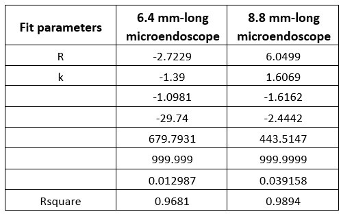
The fitting values of the parameters of equation (1) for the two lenses are reported for the Referee’s inspection here below (variables describing distances are expressed in mm):

Author response table 1.

Fitting values for the parameters of Equation (1) describing the profile of corrective microlens replicas measured with the stylus profilometer. Distances are expressed in mm.

We then assumed that the profile of the corrective microlenses were equal to the mean experimentally measured profiles and used the aspherical fitting functions in the optical simulations to compute the performance of corrected microendoscopes. For both microendoscope types, we found that the Strehl ratio was lower than 0.35, well below the theoretical diffractionlimited threshold of 0.8 (Maréchal criterion) at moderate distances from the optical axis (68 μm94 μm and 67 μm-92 μm on the focal plane in the object space, after the front end of the GRIN lens, for the 6.4 mm- and the 8.8 mm-long corrected microendoscope, respectively, Author response image 1A, C), and the PSF was strongly distorted (Author response image 1B, D).

Author response image 1.

Simulated optical performance of corrected probes with profiles of corrective microlenses equal to the mean experimentally measured profiles of fabricated corrective lenses. A) The Strehl ratio for the 6.4 mm-long corrected microendoscope with measured microlens profile (black dots) is computed on-axis (distance from the center of the FOV d = 0 µm) and at two radial distances off-axis (d = 68 μm and 94 μm on the focal plane in the object space) and compared to the Strehl ratio of the uncorrected (red line) and corrected (blue line) microendoscopes. B) Lateral (x,y) and axial (x,z) fluorescence intensity (F) profiles of simulated PSFs on-axis (left) and off-axis (right, at the indicated distance d computed on the focal plane in the object space) for the 6.4 mm-long corrected microendoscope with measured microlens profile. C) Same as in (A) for the 8.8 mm-long corrected microendoscope (off-axis d = 67 μm and 92 μm on the focal plane in the object space). D) Same as in (B) for the 8.8 mm-long corrected microendoscope.

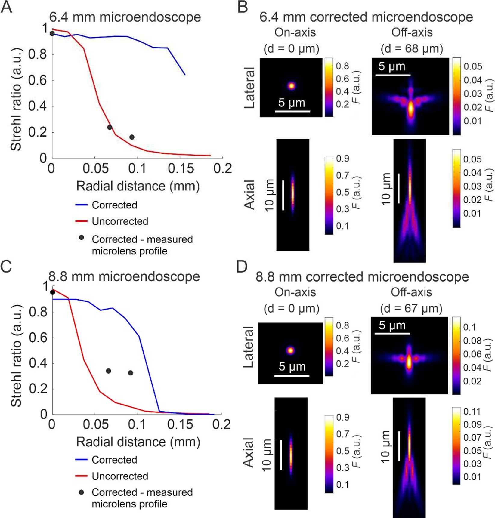
These simulated findings are in contrast with the experimentally measured optical properties of our corrected endoscopes (Figure 3). In other words, these novel simulated results show that experimentally measured profiles of the corrected lenses are incompatible with the experimental measurements of the optical properties of the corrected endoscopes. Therefore, our experimental recording of the lens profile shown in Supplementary Figure 1 of the first submission (now Supplementary Figure 4) should be used only as a coarse measure of the lens shape and cannot be used to precisely compare simulated lens profiles with measured lens profiles.

How do individual radial profiles compare to the presented means?

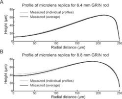
We provide below a modified version of Supplementary Figure 4 (Supplementary Figure 1 in the first submission), where individual profiles measured with the stylus profilometer and the mean profile are displayed for both microendoscope types (Author response image 2). In the manuscript (Supplementary Figure 4), we would suggest to keep showing mean profiles ± standard errors of the mean, as we did in the original submission.

Author response image 2.

Characterization of polymeric corrective lens replicas. A) Stylus profilometer measurements were performed along the radius of the corrective polymer microlens replica for the 6.4 mm-long corrected microendoscope. Individual measured profiles (grey solid lines) obtained from n = 3 profile measurements on m = 3 different corrective lens replicas, plus the mean profile (black solid line) are displayed. B) Same as (A) for the 8.8 mm-long microendoscope.

What is the practical effect of the strong field curvature? Are the edges of the field, which come very close to the lens surface, a practical limitation?

A first practical effect of the field curvature is that structures at different z coordinates are sampled. The observed field curvature of corrected endoscopes may therefore impact imaging in brain regions characterized by strong axially organized anatomy (e.g., the pyramidal layer of the hippocampus), but would not significantly affect imaging in regions with homogeneous cell density within the axial extension of the field curvature (< 170 µm, see more details below). A second consequence of the field curvature, as the Referee correctly points out, is that cell at the border of the FOV are closer to the front end of the GRIN lens. In measurements of subresolved fluorescent layers (Figure 3A-D), we observed that the field curvature extends in the axial direction to ~ 110 μm and ~170 μm for the 6.4 mm- and the 8.8 mm-long microendoscopes, respectively. Considered that the nominal working distances on the object side of the 6.4 mm- and the 8.8 mm-long microendoscopes were, respectively, 210 μm and 178 μm (Table 3), structures positioned at the very edge of the FOV were ~ 100 μm and ~ 8 μm away from the GRIN front end for the 6.4 mm-long and for the 8.8 mm-long probe, respectively. Previous studies have shown that brain tissue within 50-100 μm from the GRIN front end may show signs of tissue reaction to the implant (Curreli et al. PLOS Biology 2022, Attardo et al. Nature 2015). Therefore, structures at the very edge of the FOV of the 8.8 mm-long endoscopes, but not those at the edge of the 6.4 mm-long endoscopes, may be within the volume showing tissue reaction. We added a paragraph in the text to discuss these points (page 18 lines 10-14).

The lenses appear to be corrected for monochromatic light; high-performance microscopes are generally achromatic. Is the bandwidth of two-photon excitation sufficient to warrant optimization over multiple wavelengths?

Thanks for this comment. All optical simulations described in the first submission were performed at a fixed wavelength (λ = 920 nm). Following the Referee’s request, we explored the effect of changing wavelength on the Strehl ratio using new optical simulations. We found that the Strehl ratio remains > 0.8 at least within ± 10 nm from λ = 920 nm (new Supplementary Figure 1A-D, left panels), which covers the limited bandwidth of our femtosecond laser. Moreover, these simulations demonstrate that, on a much wider wavelength range (800 - 1040 nm), high Strehl ratio is obtained, but at different z planes (new Supplementary Figure 1A-D, right panels). This means that the corrective lens is working as expected also for wavelengths which are different from 920 nm, with different wavelengths having the most enlarged FOV located at different working distances. These new results are now described on page 7 (lines 8-10).

GRIN lenses are often used to access a 3D volume by scanning in z (including in this study). How does the corrective lens affect imaging performance over the 3D field of view?

The optical simulations we did to design the corrective lenses were performed maximizing aberration correction only in the focal plane of the endoscope. Following the Referee’s comment, we explored the effect of aberration correction outside the focal plane using new optical simulations. In corrected endoscopes, we found that for off-axis rays (radial distance from the optical axis > 40 μm) the Strehl ratio was > 0.8 (Maréchal criterion) in a larger volume compared to uncorrected endoscopes (new Supplementary Figure 2), demonstrating that the aberration correction method developed in this study does extend beyond the focal plane for short distances. For example, at a radial distance of ~ 90 μm from the optical axis, the axial range in which the Strehl ratio was > 0.8 in corrected endoscopes was 28 μm and 19 μm for the 6.4 mm- and the 8.8 mm-long microendoscope, respectively. These new results are now described on page 7 (10-19).

(4) The in vivo images (Figure 7D) have a less impressive resolution and field than the ex vivo images (Figure 4B), and the reason for this is not clear. Given the difference in performance, how does this compare to an uncorrected endoscope in the same preparation? Is the reduced performance related to uncorrected motion, field curvature, working distance, etc?

In comparing images in Figure 4B with images shown in Figure 7D, the following points should be considered:

(1) Figure 4B is a maximum fluorescence intensity projection of multiple axial planes of a z-stack acquired through a thin brain slice (slice thickness: 50 µm) using 8 frame averages for each plane. In contrast, images in Figure 7D are median projection of a t-series acquired on a single plane in the awake mouse at 30 Hz resonant scanning imaging (8 min, 14,400 frames).

(2) Images of the fixed brain slice in Figure 4B were acquired at 1024 pixels x 1024 pixels resolution, nominal pixel size 0.45 µm/pixel, and with objective NA = 0.50, whereas in vivo images in Figure 7D were acquired at 512 pixels x 512 pixels resolution, nominal pixel size 0.72 - 0.84 µm/pixel, and with objective NA = 0.45.

(3) In the in vivo preparation (Figure 7D), excitation and emission light travel through > 180 µm of scattering and absorbing brain tissue, reducing spatial resolution and the SNR of the collected fluorescence signal.

(4) By shifting the sample in the x, y plane, in Figure 4B we could chose a FOV containing homogenously stained cells. x, y shifting and selecting across multiple FOVs was not possible in vivo, as the GRIN lens was cemented on the animal skull.

(5) Images in Figure 7D were motion corrected, but we cannot exclude that part of the decrease in resolution observed in Figure 7D when compared to images in Figure 4B are due to incomplete correction of motion artifacts.

For all the reasons listed above, we believe that it is expected to see smaller resolution and contrast in images recorded in vivo (Figure 7D) compared to images acquired in fixed tissue (Figure 4B).

Regarding the question of how do images from an uncorrected and a corrected endoscopes compared in vivo, we think that this comparison is better performed in fixed tissue (Figure 4) or in simulated calcium data (Figure 5-6), rather than in vivo recordings (Figure 7). In fact, in the brain of living mice motion artifacts, changes in fluorophore expression level, variation in the optical properties of the brain (e.g., the presence of a blood vessel over the FOV) may make the comparison of images acquired with uncorrected and corrected microendoscopes difficult, requiring a large number of animals to cancel out the contributions of these factors. Comparing optical properties in fixed tissue is, in contrast, devoid of these confounding factors. Moreover, the major advantage of quantifying how the optical properties of uncorrected and corrected endoscopes impact on the ability to extract information about neuronal activity in simulated calcium data is that, under simulated conditions, we can count on a known ground truth as reference (e.g., how many neurons are in the FOV, where they are, and which is their electrical activity). This is clearly not possible in the in vivo recordings.

Regarding Figure 7, there is no analysis of the biological significance of the calcium signals or even a description of where olfactory stimuli were presented.

We appreciate the Reviewer pointing out the lack of detailed analysis regarding the biological significance of the calcium signals and the presentation of olfactory stimuli in Figure 7. Our initial focus was on demonstrating the effectiveness of the optimized GRIN lenses for imaging deep brain areas like the piriform cortex, with an emphasis on the improved signal-tonoise ratio (SNR) these lenses provide. However, we agree that including more context about the experimental conditions would enhance the manuscript. To address this point, we added a new panel (Figure 7F) showing calcium transients aligned with the onset of olfactory stimulus presentations, which are now indicated by shaded light blue areas. Additionally, we have specified the timing of each stimulus presented in Figure 7E. This revision allows readers to better understand the relationship between the calcium signals and the olfactory stimuli.

The timescale of jGCaMP8f signals in Figure 7E is uncharacteristically slow for this indicator (compared to Zhang et al 2023 (Nature)), though perhaps this is related to the physiology of these cells or the stimuli.

Regarding the timescale of the calcium signals observed in Figure 7E, we apologize for the confusion caused by a mislabeling we inserted in the original manuscript. The experiments presented in Figure 7 were conducted using jGCaMP7f, not jGCaMP8f as previously stated (both indicators were used in this study but in separate experiments). We have corrected this error in the Results section (caption of Figure 7D, E). It is important to note that jGCaMP7f has a longer half-decay time compared to jGCaMP8f, which could in part account for the slower decay kinetics observed in our data. Furthermore, the prolonged calcium signals can be attributed to the physiological properties of neurons in the piriform cortex. Upon olfactory stimulation, these neurons often fire multiple action potentials, resulting in extended calcium transients that can last several seconds. This sustained activity has been documented in previous studies, such as Roland et al. (eLife 2017, Figure 1C therein) in anesthetized animals and Wang et al. (Neuron 2020, Figure 1E therein) in awake animals, which report similar durations for calcium signals.

(5) The claim of unprecedented spatial resolution across the FOV (page 18) is hard to evaluate and is not supported by references to quantitative comparisons. The promises of the method for future studies (pages 18-19) could also be better supported by analysis or experiment, but these are minor and to me, do not detract from the appeal of the work.

GRIN lens-based imaging of piriform cortex in the awake mouse had already been done in Wang et al., Neuron 2020. The GRIN lens used in that work was NEM-050-50-00920-S-1.5p (GRINTECH, length: 6.4 mm; diameter: 0.5 mm), similar to the one that we used to design the 6.4 mm-long corrected microendoscope. Here we used a microendoscope specifically design to correct off-axis aberrations and enlarge the FOV, in order to maximize the number of neurons recorded with the highest possible spatial resolution, while keeping the tissue invasiveness to the minimum. Following the Referee’s comments, we revised the sentence at page 19 (lines 68 from bottom) as follows:

“We used long corrected microendoscopes to measure population dynamics in the olfactory cortex of awake head-restrained mice with unprecedented combination of high spatial resolution across the FOV and minimal invasiveness(17)”.

(6) The text is lengthy and the material is repeated, especially between the introduction and conclusion. Consolidating introductory material to the introduction would avoid diluting interesting points in the discussion.

We thank the Reviewer for this comment. As suggested, we edited the Introduction and shortened the Discussion.

Reviewer #2 (Public review):

In this manuscript, the authors present an approach to correct GRIN lens aberrations, which primarily cause a decrease in signal-to-noise ratio (SNR), particularly in the lateral regions of the field-of-view (FOV), thereby limiting the usable FOV. The authors propose to mitigate these aberrations by designing and fabricating aspherical corrective lenses using ray trace simulations and two-photon lithography, respectively; the corrective lenses are then mounted on the back aperture of the GRIN lens.

This approach was previously demonstrated by the same lab for GRIN lenses shorter than 4.1 mm (Antonini et al., eLife, 2020). In the current work, the authors extend their method to a new class of GRIN lenses with lengths exceeding 6 mm, enabling access to deeper brain regions as most ventral regions of the mouse brain. Specifically, they designed and characterized corrective lenses for GRIN lenses measuring 6.4 mm and 8.8 mm in length. Finally, they applied these corrected long micro-endoscopes to perform high-precision calcium signal recordings in the olfactory cortex.

Compared with alternative approaches using adaptive optics, the main strength of this method is that it does not require hardware or software modifications, nor does it limit the system's temporal resolution. The manuscript is well-written, the data are clearly presented, and the experiments convincingly demonstrate the advantages of the corrective lenses.

The implementation of these long corrected micro-endoscopes, demonstrated here for deep imaging in the mouse olfactory bulb, will also enable deep imaging in larger mammals such as rats or marmosets.

We thank the Referee for the positive comments on our study. We address the points indicated by the Referee in the “Recommendation to the authors” section below.

Reviewer #3 (Public review):

Summary:

This work presents the development, characterization, and use of new thin microendoscopes (500µm diameter) whose accessible field of view has been extended by the addition of a corrective optical element glued to the entrance face. Two micro endoscopes of different lengths (6.4mm and 8.8mm) have been developed, allowing imaging of neuronal activity in brain regions >4mm deep. An alternative solution to increase the field of view could be to add an adaptive optics loop to the microscope to correct the aberrations of the GRIN lens. The solution presented in this paper does not require any modification of the optical microscope and can therefore be easily accessible to any neuroscience laboratory performing optical imaging of neuronal activity.

Strengths:

(1) The paper is generally clear and well-written. The scientific approach is well structured and numerous experiments and simulations are presented to evaluate the performance of corrected microendoscopes. In particular, we can highlight several consistent and convincing pieces of evidence for the improved performance of corrected micro endoscopes:

a) PSFs measured with corrected micro endoscopes 75µm from the centre of the FOV show a significant reduction in optical aberrations compared to PSFs measured with uncorrected micro endoscopes.

b) Morphological imaging of fixed brain slices shows that optical resolution is maintained over a larger field of view with corrected micro endoscopes compared to uncorrected ones, allowing neuronal processes to be revealed even close to the edge of the FOV.

c) Using synthetic calcium data, the authors showed that the signals obtained with the corrected microendoscopes have a significantly stronger correlation with the ground truth signals than those obtained with uncorrected microendoscopes.

(2) There is a strong need for high-quality micro endoscopes to image deep brain regions in vivo. The solution proposed by the authors is simple, efficient, and potentially easy to disseminate within the neuroscience community.

Weaknesses:

(1) Many points need to be clarified/discussed. Here are a few examples:

a) It is written in the methods: “The uncorrected microendoscopes were assembled either using different optical elements compared to the corrected ones or were obtained from the corrected

probes after the mechanical removal of the corrective lens.”

This is not very clear: the uncorrected microendoscopes are not simply the unmodified GRIN lenses?

We apologize for not been clear enough on this point. Uncorrected microendoscopes are not simply unmodified GRIN lenses, rather they are GRIN lenses attached to a round glass coverslip (thickness: 100 μm). The glass coverslip was included in ray-trace optical simulations of the uncorrected system and this is the reason why commercial GRIN lenses and corresponding uncorrected microendoscopes have different working distances, as reported in Tables 2-3. To make the text clearer, we added the following sentence at page 27 (last 4 lines):

“To evaluate the impact of corrective microlenses on the optical performance of GRIN-based microendoscopes, we also simulated uncorrected microendoscopes composed of the same optical elements of corrected probes (glass coverslip and GRIN rod), but in the absence of the corrective microlens”.

b) In the results of the simulation of neuronal activity (Figure 5A, for example), the neurons in the center of the FOV have a very large diameter (of about 30µm). This should be discussed.

Thanks for this comment. In synthetic calcium imaging t-series, cell radii were randomly sampled from a Gaussian distribution with mean = 10 µm and standard deviation (SD) = 3 µm. Both values were estimated from the literature (ref. no. 28: Suzuki & Bekkers, Journal of Neuroscience, 2011) as described in the Methods (page 35). In the image shown in Figure 5A, neurons near to the center of the FOV have radius of ~ 20 µm corresponding to the right tail of the distribution (mean + 3SD = 19 µm). It is also important to note that, for corrected microendoscopes, neurons in the central portion of the FOV appear larger than cells located near the edges of the FOV, because the magnification depends on the distance from the optical axis (see Figure 3E, F) and near the center the magnification is > 1 for both microendoscope types.

Also, why is the optical resolution so low on these images?

Images shown in Figure 5 are median fluorescence intensity projections of 5 minute-long simulated t-series. Simulated calcium data were generated with pixel size 0.8 μm/pixel and frame rate 30 Hz, similarly to in vivo recordings. In the simulations, pixels not belonging to any cell soma were assigned a value of background fluorescence randomly sampled from a normal distribution with mean and standard deviation estimated from experimental data, as described in the Methods section (page 37). To simulate activity, the mean spiking rate of neurons was set to 0.3 Hz, thus in a large fraction of frames neurons do not show calcium transients. Therefore, the median fluorescence intensity value of somata will be close to their baseline fluorescence value (_F_0). Since in simulations F0 values (~ 45-80 a.u.) were not much higher than the background fluorescence level (~ 45 a.u.), this may generate the appearance of low contrast image in Figure 5A. Finally, we suspect that PDF rendering also contributed to degrade the quality of those images. We will now submit high resolution images alongside the PDF file.

c) It seems that we can't see the same neurons on the left and right panels of Figure 5D. This should be discussed.

The Referee is correct. When we intersected the simulated 3D volume of ground truth neurons with the focal surface of microendoscopes, the center of the FOV for the 8.8 mmlong corrected microendoscope was located at a larger depth than the FOV of the 8.8 mm uncorrected microendoscope. This effect was due to the larger field curvature of corrected 8.8 mmlong endoscopes compared to 8.8 mm-long uncorrected endoscopes. This is the reason why different neurons were displayed for uncorrected and corrected endoscopes in Figure 5D. We added this explanation in the text at page 37 (lines 1-4). The text reads:

“Due to the stronger field curvature of the 8.8 mm-long corrected microendoscope (Figure 1C) compared to 8.8 mm-long uncorrected microendoscopes, the center of the corrected imaging focal surface resulted at a larger depth in the simulated volume compared to the center of the uncorrected focal surface(s). Therefore, different simulated neurons were sampled in the two cases”.

d) It is not very clear to me why in Figure 6A, F the fraction of adjacent cell pairs that are more correlated than expected increases as a function of the threshold on peak SNR. The authors showed in Supplementary Figure 3B that the mean purity index increases as a function of the threshold on peak SNR for all micro endoscopes. Therefore, I would have expected the correlation between adjacent cells to decrease as a function of the threshold on peak SNR. Similarly, the mean purity index for the corrected short microendoscope is close to 1 for high thresholds on peak SNR: therefore, I would have expected the fraction of adjacent cell pairs that are more correlated than expected to be close to 0 under these conditions. It would be interesting to clarify these points.

Thanks for raising this point. We defined the fraction of adjacent cell pairs more correlated than expected as the number of adjacent cell pairs more correlated than expected divided by the number of adjacent cell pairs. The reason why this fraction raises as a function of the SNR threshold is shown in Supplementary Figure 2 in the first submission (now Supplementary Figure 5). There, we separately plotted the number of adjacent cell pairs more correlated than expected (numerator) and the number of adjacent cell pairs (denominator) as a function of the SNR threshold. For both microendoscope types, we observed that the denominator more rapidly decreased with peak SNR threshold than the numerator. Therefore, the fraction of adjacent cell pairs more correlated than expected increases with the peak SNR threshold.

To understand why the denominator decreases with SNR threshold, it should be considered that, due to the deterioration of spatial resolution and attenuation of fluorescent signal collection as a function of the radial distance from the optical axis (see for example fluorescent film profiles in Figure 3A, C), increasing the threshold on the peak SNR of extracted calcium traces implies limiting cell detection to those cells located within smaller distance from the center of the FOV. This information is shown in Figure 5C, F.

In the manuscript text, this point is discussed at page 12 (lines 1-3 from bottom) and page 13 (lines 1-4):

“The fraction of pairs of adjacent cells (out of the total number of adjacent pairs) whose activity correlated significantly more than expected increased as a function of the SNR threshold for corrected and uncorrected microendoscopes of both lengths (Fig. 6A, F). This effect was due to a larger decrease of the total number of pairs of adjacent cells as a function of the SNR threshold compared to the decrease in the number of pairs of adjacent cells whose activity was more correlated than expected (Supplementary Figure 5)”.

e) Figures 6C, H: I think it would be fairer to compare the uncorrected and corrected endomicroscopes using the same effective FOV.

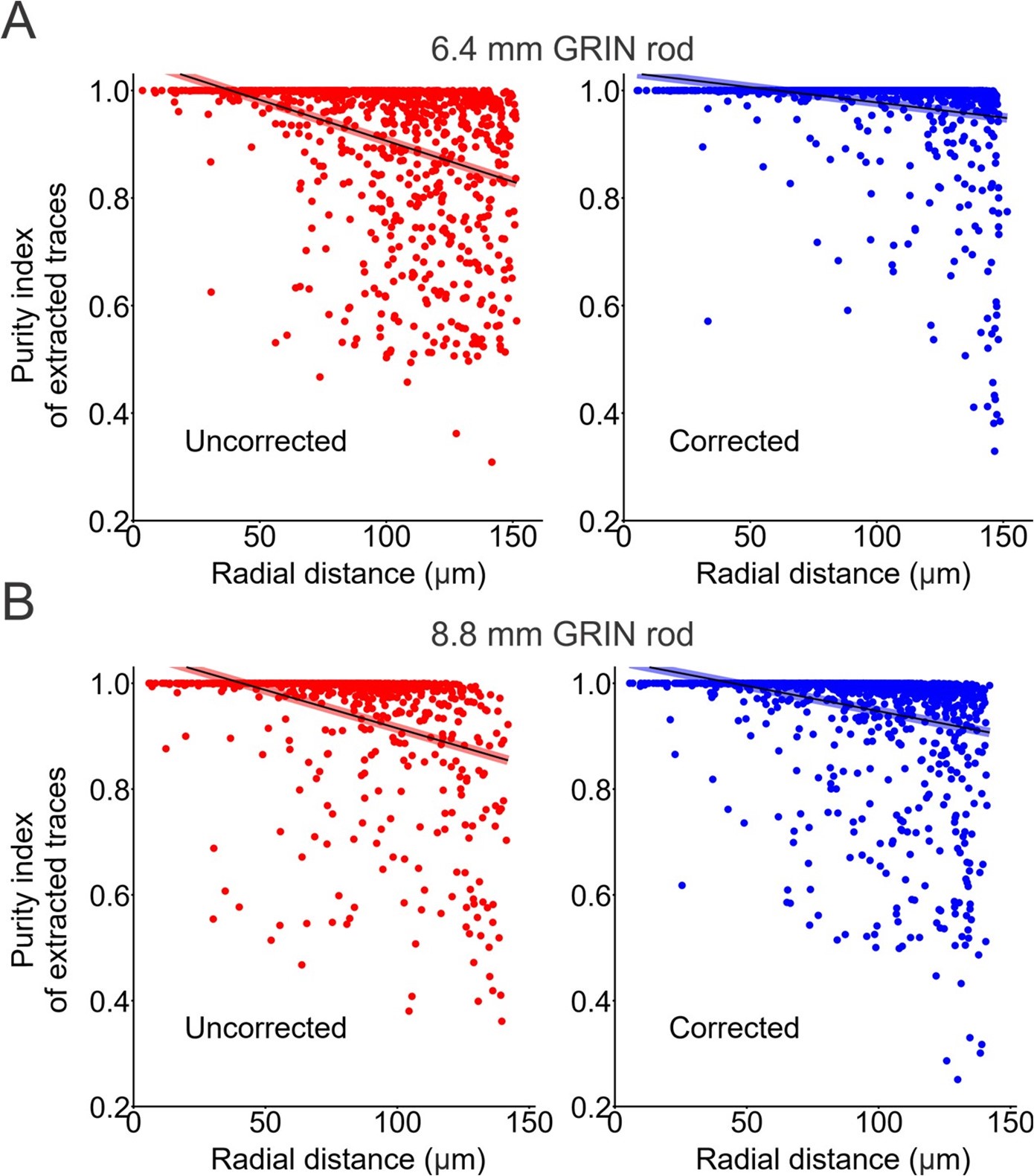
To address the Reviewer’s concern, we repeated the linear regression of purity index as a function of the radial distance using the same range of radial distances for the uncorrected and corrected case of both microendoscope types. Below, we provide an updated version of Figure 6C, H for the referee’s perusal. Please note that the maximum value displayed on the x-axis of both graphs is now corresponding to the minimum value between the two maximum radial distance values obtained in the uncorrected and corrected case (maximum radial distance displayed: 151.6 µm and 142.1 μm for the 6.4 mm- and the 8.8 mm-long GRIN rod, respectively). Using the same effective FOV, we found that the purity index drops significantly more rapidly with the radial distance for uncorrected microendoscopes compared to the corrected ones, similarly to what observed in the original version of Figure 6. The values of the linear regression parameters and statistical significance of the difference between the slopes in the uncorrected and corrected cases are stated in the Author response image 3 caption below for both microendoscope types. In the manuscript, we would suggest to keep showing data corresponding to all detected cells, as we did in the original submission.

Author response image 3.

Linear regression of purity index as a function of the radial distance. A) Purity index of extracted traces with peak SNR > 10 was estimated using a GLM of ground truth source contributions and plotted as a function of the radial distance of cell identities from the center of the FOV for n = 13 simulated experiments with the 6.4 mm-long uncorrected (red) and corrected (blue) microendoscope. Black lines represent the linear regression of data ± 95% confidence intervals (shaded colored areas). Maximum value of radial distance displayed: 151.6 μm. Slopes ± standard error (s.e.): uncorrected, (-0.0015 ± 0.0002) µm-1; corrected, (-0.0006 ± 0.0001) μm-1. Uncorrected, n = 991; corrected, n = 1156. Statistical comparison of slopes, p < 10^-10, permutation test. B) Same as (A) for n = 15 simulated experiments with the 8.8 mm-long uncorrected and corrected microendoscope. Maximum value of radial distance displayed: 142.1 μm. Slopes ± s.e.: uncorrected, (-0.0014 ± 0.0003) μm-1; corrected, (-0.0010 ± 0.0002) µm-1. Uncorrected, n = 718; corrected, n = 1328. Statistical comparison of slopes, p = 0.0082, permutation test.

f) Figure 7E: Many calcium transients have a strange shape, with a very fast decay following a plateau or a slower decay. Is this the result of motion artefacts or analysis artefacts?

Thank you for raising this point about the unusual shapes of the calcium transients in Figure 7E. The observed rapid decay following a plateau or a slower decay is indeed a result of how the data were presented in the original submission. Our experimental protocol consisted of 22 s-long trials with an inter-trial interval of 10 s (see Methods section, page 44). In the original figure, data from multiple trials were concatenated, which led to artefactual time courses and apparent discontinuities in the calcium signals. To resolve this issue, we revised Figure 7E to accurately represent individual concatenated trials. We also added a new panel (please see new Figure 7F) showing examples of single cell calcium responses in individual trials without concatenation, with annotations indicating the timing and identity of presented olfactory stimuli.

Also, the duration of many calcium transients seems to be long (several seconds) for GCaMP8f. These points should be discussed.

Author response: regarding the timescale of the calcium signals observed in Figure 7E, we apologize for the confusion caused by a mislabeling we inserted in the manuscript. The experiments presented in Figure 7 were conducted using jGCaMP7f, not jGCaMP8f as previously stated (both indicators were used in this study, but in separate experiments). We have corrected this error in the Results section (caption of Figure 7D, E). It is important to note that jGCaMP7f has a longer half-decay time compared to jGCaMP8f, which could in part account for the slower decay kinetics observed in our data. Furthermore, the prolonged calcium signals can be attributed to the physiological properties of neurons in the piriform cortex. Upon olfactory stimulation, these neurons often fire multiple action potentials, resulting in extended calcium transients that can last several seconds. This sustained activity has been documented in previous studies, such as Roland et al. (eLife 2017, Figure 1C therein) in anesthetized animals and Wang et al. (Neuron 2020, Figure 1E therein) in awake animals, which report similar durations for calcium signals. We cite these references in the text. We believe that these revisions and clarifications address the Reviewer's concern and enhance the overall clarity of our manuscript.

g) The authors do not mention the influence of the neuropil on their data. Did they subtract the neuropil's contribution to the signals from the somata? It is known from the literature that the presence of the neuropil creates artificial correlations between neurons, which decrease with the distance between the neurons (Grødem, S., Nymoen, I., Vatne, G.H. et al. An updated suite of viral vectors for in vivo calcium imaging using intracerebral and retro-orbital injections in male mice. Nat Commun 14, 608 (2023). https://doi.org/10.1038/s41467-023-363243; Keemink SW, Lowe SC, Pakan JMP, Dylda E, van Rossum MCW, Rochefort NL. FISSA: A neuropil decontamination toolbox for calcium imaging signals. Sci Rep. 2018 Feb 22;8(1):3493.

doi: 10.1038/s41598-018-21640-2. PMID: 29472547; PMCID: PMC5823956)

This point should be addressed.

We apologize for not been clear enough in our previous version of the manuscript. The neuropil was subtracted from calcium traces both in simulated and experimental data. Please note that instead of using the term “neuropil”, we used the word “background”. We decided to use the more general term “background” because it also applies to the case of synthetic calcium tseries, where neurons were modeled as spheres devoid of processes. The background subtraction is described in the Methods on page 39:

“F(t) was computed frame-by-frame as the difference between the average signal of pixels in each ROI and the background signal. The background was calculated as the average signal of pixels that: i) did not belong to any bounding box; ii) had intensity values higher than the mean noise value measured in pixels located at the corners of the rectangular image, which do not belong to the circular FOV of the microendoscope; iii) had intensity values lower than the maximum value of pixels within the boxes”.

h) Also, what are the expected correlations between neurons in the pyriform cortex? Are there measurements in the literature with which the authors could compare their data?

We appreciate the reviewer's interest in the correlations between neurons in the piriform cortex. The overall low correlations between piriform neurons we observed (Figure 8) are consistent with a published study describing ‘near-zero noise correlations during odor inhalation’ in the anterior piriform cortex of rats, based on extracellular recordings (Miura et al., Neuron 2013). However, to the best of our knowledge, measurements directly comparable to ours have not been described in the literature. Recent analyses of the correlations between piriform neurons were restricted to odor exposure windows, with the goal to quantify odor-specific activation patterns (e.g. Roland et al., eLife 2017; Bolding et al., eLife 2017, Pashkovski et al., Nature 2020; Wang et al., Neuron 2020). Here, we used correlation analyses to characterize the technical advancement of the optimized GRIN lens-based endoscopes. We showed that correlations of pairs of adjacent neurons were independent from radial distance (Figure 8B), highlighting homogeneous spatial resolution in the field of view.

(2) The way the data is presented doesn't always make it easy to compare the performance of corrected and uncorrected lenses. Here are two examples:

a) In Figures 4 to 6, it would be easier to compare the FOVs of corrected and uncorrected lenses if the scale bars (at the centre of the FOV) were identical. In this way, the neurons at the centre of the FOV would appear the same size in the two images, and the distances between the neurons at the centre of the FOV would appear similar. Here, the scale bar is significantly larger for the corrected lenses, which may give the illusion of a larger effective FOV.

We appreciate the Referee’s comment. Below, we explain why we believe that the way we currently present imaging data in the manuscript is preferable:

(1) current figures show images of the acquired FOV as they are recorded from the microscope (raw data), without rescaling. In this way, we exactly show what potential users will obtain when using a corrected microendoscope.

(2) In the current version of the figures, the fact that the pixel size is not homogeneous across the FOV, nor equal between uncorrected and corrected microendoscopes, is initially shown in Figure 3E, F and then explicitly stated throughout the manuscript when images acquired with a corrected microendoscope are shown.

(3) Rescaling images acquired with the corrected endoscopes gives the impression that the acquisition parameters were different between acquisitions with the corrected and uncorrected microendoscopes, which was not the case.

Importantly, the larger FOV of the corrected microendoscope, which is one of the important technological achievements presented in this study, can be appreciated in the images regardless of the presentation format.

b) In Figures 3A-D it would be more informative to plot the distances in microns rather than pixels. This would also allow a better comparison of the micro endoscopes (as the pixel sizes seem to be different for the corrected and uncorrected micro endoscopes).

The Referee is correct that the pixel size is different between the corrected and uncorrected probes. This is because of the different magnification factor introduced by the corrective microlens, as described in Figure 3E, F. The rationale for showing images in Figure 3AD in pixels rather than microns is the following:

(1) Optical simulations in Figure 1 suggest that a corrective optical element is effective in compensating for some of the optical aberrations in GRIN microendoscopes.

(2) After fabricating the corrective optical element (Figure 2), in Figure 3A-D we conduct a preliminary analysis of the effect of the corrective optical element on the optical properties of the GRIN lens. We observed that the microfabricated optical element corrected for some aberrations (e.g., astigmatism), but also that the microfabricated optical element was characterized by significant field curvature. This can be appreciated showing distances in pixels.

(3) The observed field curvature and the aspherical profile of the corrected lens prompted us to characterize the magnification factor of the corrected endoscopes as a function of the radial distance. We found that the magnification factor changed as a function of the radial distance (Figure 3E-F) and that pixel size was different between uncorrected and corrected endoscopes. We also observed that, in corrected endoscopes, pixel size was a function of the radial distance (Figure 3E-F).

(4) Once all of the above was established and quantified, we assigned precise pixel size to images of uncorrected and corrected endoscopes and we show all following images of the study (Figure 3G on) using a micron (rather than pixel) scale.

(3) There seems to be a discrepancy between the performance of the long lenses (8.8 mm) in the different experiments, which should be discussed in the article. For example, the results in Figure 4 show a considerable enlargement of the FOV, whereas the results in Figure 6 show a very moderate enlargement of the distance at which the person's correlation with the first ground truth emitter starts to drop.

Thanks for raising this point and helping us clarifying data presentation. Images in Figure 4B are average z-projections of z-stacks acquired through a mouse fixed brain slice and they were taken with the purpose of showing all the neurons that could be visualized from the same sample using an uncorrected and a corrected microendoscope. In Figure 4B, all illuminated neurons are visible regardless of whether they were imaged with high axial resolution (e.g., < 10 µm as defined in Figure 3J) or poor axial resolution. In contrast, in Figure 6J we evaluated the correlation between the calcium trace extracted from a given ROI and the real activity trace of the first simulated ground truth emitter for that specific ROI. The moderate increase in the correlation for the corrected microendoscope compared to the uncorrected microendoscope (Figure 6J) is consistent with the moderate improvement in the axial resolution of the corrected probe compared to the uncorrected probe at intermediate radial distances (60-100 µm from the optical axis, see Figure 3J). We added a paragraph in the Results section (page 14, lines 8-18) to summarize the points described above.

a) There is also a significant discrepancy between measured and simulated optical performance, which is not discussed. Optical simulations (Figure 1) show that the useful FOV (defined as the radius for which the size of the PSF along the optical axis remains below 10µm) should be at least 90µm for the corrected microendoscopes of both lengths. However, for the long microendoscopes, Figure 3J shows that the axial resolution at 90µm is 17µm. It would be interesting to discuss the origin of this discrepancy: does it depend on the microendoscope used?

As the Reviewer correctly pointed out, the size of simulated PSFs at a given radial distance (e.g., 90 µm) tends to be generally smaller than that of the experimentally measured PSFs. This might be due to multiple reasons:

(1) simulated PSFs are excitation PSFs, i.e. they describe the intensity spatial distribution of focused excitation light. On the contrary, measured PSFs result from the excitation and emission process, thus they are also affected by aberrations of light emitted by fluorescent beads and collected by the microscope.

(2) in the optical simulations, the Zemax file of the GRIN lenses contained first-order aberrations. High-order aberrations were therefore not included in simulated PSFs.

(3) intrinsic variability of experimental measurements (e.g., intrinsic variability of the fabrication process, alignment of the microendoscope to the optical axis of the microscope, the distance between the GRIN back end and the objective…) are not considered in the simulations.

We added a paragraph in the Discussion section (page 17, lines 9-18) summarizing the abovementioned points.

Are there inaccuracies in the construction of the aspheric corrective lens or in the assembly with the GRIN lens? If there is variability between different lenses, how are the lenses selected for imaging experiments?

The fabrication yield, i.e. the yield of generating the corrective lenses, using molding was ~ 90% (N > 30 molded lenses). The main limitation of this procedure was the formation of air bubbles between the mold negative and the glass coverslip. Molded lenses were visually inspected with the stereoscope and, in case of air bubble formation, they were discarded.

The assembly yield, i.e. the yield of correct positioning of the GRIN lens with respect to the coverslip, was 100 % (N = 27 endoscopes).

We added this information in the Methods at page 29 (lines 1-12), as follows:

“After UV curing, the microlens was visually inspected at the stereomicroscope. In case of formation of air bubbles, the microlens was discarded (yield of the molding procedure: ~ 90 %, N > 30 molded lenses). The coverslip with the attached corrective lens was sealed to a customized metal or plastic support ring of appropriate diameter (Fig. 2C). The support ring, the coverslip and the aspherical lens formed the upper part of the corrected microendoscope, to be subsequently coupled to the proper GRIN rod (Table 2) using a custom-built opto-mechanical stage and NOA63 (Fig. 2C) 7. The GRIN rod was positioned perpendicularly to the glass coverslip, on the other side of the coverslip compared to the corrective lens, and aligned to the aspherical lens perimeter (Fig. 2C) under the guidance of a wide field microscope equipped with a camera. The yield of the assembly procedure for the probes used in this work was 100 % (N = 27 endoscopes). For further details on the assembly of corrected microendoscope see(7)”.

Reviewer #1 (Recommendations for the authors):

(1) Page 4, what is meant by 'ad-hoc" in describing software control?

With “ad-hoc” we meant “specifically designed”. We revised the text to make this clear.

(2) It was hard to tell how the PSF was modeled for the simulations (especially on page 34, describing the two spherical shells of the astigmatic PSF and ellipsoids modeled along them). Images or especially videos that show the modeling would make this easier to follow.

Simulated calcium t-series were generated following previous work by our group (Antonini et al., eLife 2020), as stated in the Methods on page 37 (line 5). In Figure 4A of Antonini et al. eLife 2020, we provided a schematic to visually describe the procedure of simulated data generation. In the present paper, we decided not to include a similar drawing and cite the eLife 2020 article to avoid redundancy.

(3) Some math symbols are missing from the methods in my version of the text (page 36/37).

We apologize for the inconvenience. This issue arose in the PDF conversion of our Word document and we did not spot it at the time of submission. We will now make sure the PDF version of our manuscript correctly reports symbols and equations.

(4) The Z extent of stacks (i.e. number of steps) used to generate images in Figure 4 is missing.

We thank the Reviewer for the comment and we now revised the caption of Figure 4 and the Methods section as follows:

“Figure 4. Aberration correction in long GRIN lens-based microendoscopes enables highresolution imaging of biological structures over enlarged FOVs. A) jGCaMP7f-stained neurons in a fixed mouse brain slice were imaged using 2PLSM (λexc = 920 nm) through an uncorrected (left) and a corrected (right) microendoscope based on the 6.4 mm-long GRIN rod. Images are maximum fluorescence intensity (F) projections of a z-stack acquired with a 5 μm step size. Number of steps: 32 and 29 for uncorrected and corrected microendoscope, respectively. Scale bars: 50 μm. Left: the scale applies to the entire FOV. Right, the scale bar refers only to the center of the FOV; off-axis scale bar at any radial distance (x and y axes) is locally determined multiplying the length of the drawn scale bar on-axis by the corresponding normalized magnification factor shown in the horizontal color-coded bar placed below the image (see also Fig. 3, Supplementary Table 3, and Materials and Methods for more details). B) Same results for the microendoscope based on the 8.8 mm-long GRIN rod. Number of steps: 23 and 31 for uncorrected and corrected microendoscope, respectively”.

We also modified the text in the Methods (page 35, lines 1-2):

“(1024 pixels x 1024 pixels resolution; nominal pixel size: 0.45 µm/pixel; axial step: 5 µm; number of axial steps: 23-32; frame averaging = 8)”.

(5) Overall, the text is wordy and a bit repetitive and could be cut down significantly in length without loss of clarity. This is true throughout, but especially when comparing the introduction and discussion.

We edited the text (Discussion and Introduction), as suggested by the Reviewer.

(6) Although I don't think it's necessary, I would advise including comparison data with an uncorrected endoscope in the same in vivo preparation.

We thank the Referee for the suggestion. Below, we list the reasons why we decided not to perform the comparison between the uncorrected and corrected endoscopes in the in vivo preparation:

(1) We believe that the comparison between uncorrected and corrected endoscopes is better performed in fixed tissue (Figure 4) or in simulated calcium data (Figure 5-6), rather than in vivo recordings (Figure 7). In fact, in the brain of living mice motion artifacts, changes in fluorophore expression level, variation in the optical properties of the brain (e.g., the presence of a blood vessel over the FOV) may make the comparison of images acquired with uncorrected and corrected microendoscopes difficult, requiring a large number of animals to cancel out the contributions of all these factors. Comparing optical properties in fixed tissue is, in contrast, devoid of these confounding factors.

(2) A major advantage of quantifying how the optical properties of uncorrected and corrected endoscope impact on the ability to extract information about neuronal activity in simulated calcium data is that, under simulated conditions, we can count on a known ground truth as reference (e.g., how many neurons are in the FOV, where they are, and which is their electrical activity). This is clearly not possible under in vivo conditions.

(3) The proposed experiment requires to perform imaging in the awake mouse with a corrected microendoscope, then anesthetize the animal to carefully remove the corrective microlens using forceps, and finally repeat the optical recordings in awake mice with the uncorrected microendoscope. Although this is feasible (we performed the proposed experiment in Antonini et al. eLife 2020 using a 4.1 mm-long microendoscope), the yield of success of these experiments is low. The low yield is due to the fact that the mechanical force applied on top of the microendoscope to remove the corrective microlens may induce movement of the GRIN lens inside the brain, both in vertical and horizontal directions. This can randomly result in change of the focal plane, death or damage of the cells, tissue inflammation, and bleeding. From our own experience, the number of animals used for this experiment is expected to be high.

Reviewer #2 (Recommendations for the authors):

Below, I provide a few minor corrections and suggestions for the authors to consider before final submission.

(1) Page 5: when referring to Table 1 maybe add "Table 1 and Methods".

Following the Reviewer’s comment, we revised the text at page 6 (lines 4-5 from bottom) as follows:

“(see Supplementary Table 1 and Materials and Methods for details on simulation parameters)”.

(2) Page 8: "We set a threshold of 10 µm on the axial resolution to define the radius of the effective FOV (corresponding to the black triangles in Fig. 3I, J) in uncorrected and corrected microendoscopes. We observed an enlargement of the effective FOV area of 4.7 times and 2.3 times for the 6.4 mm-long micro endoscope and the 8.8 mm-long micro endoscope, respectively (Table 1). These findings were in agreement with the results of the ray-trace simulations (Figure 1) and the measurement of the subresolved fluorescence layers (Figure 3AD)." I could not find the information given in this paragraph, specifically:

a) Upon examining the black triangles in Figure 3I and J, the enlargement of the effective FOV does not appear to be 4.7 and 2.3 times.

In Figure 3I, J, black triangles mark the intersections between the curves fitting the data and the threshold of 10 µm on the axial resolution. The values on the x-axis corresponding to the intersections (Table 1, “Effective FOV radius”) represent the estimated radius of the effective FOV of the probes, i.e. the radius within which the microendoscope has spatial resolution below the threshold of 10 μm. The ratios of the effective FOV radii are 2.17 and 1.53 for the 6.4 mm- and the 8.8 mm-long microendoscope, respectively, which correspond to 4.7 and 2.3 times larger FOV (Table 1). To make this point clearer, we modified the indicated sentence as follows (page 10, lines 3-11 from bottom):

“We set a threshold of 10 µm on the axial resolution to define the radius of the effective FOV (corresponding to the black triangles in Fig. 3I, J) in uncorrected and corrected microendoscopes. We observed a relative increase of the effective FOV radius of 2.17 and 1.53 for the 6.4 mm- and the 8.8 mm-long microendoscope, respectively (Table 1). This corresponded to an enlargement of the effective FOV area of 4.7 times and 2.3 times for the 6.4 mm-long microendoscope and the 8.8

mm-long microendoscope, respectively (Table 1). These findings were in agreement with the results of the ray-trace simulations (Figure 1) and the measurement of the subresolved fluorescence layers (Figure 3A-D)."

b) I do not understand how the enlargements in Figure 3I and J align with the ray trace simulations in Figure 1, indicating an enlargement of 5.4 and 5.6.

In Figure 1C, E of the first submission we showed the Strehl ratio of focal spots focalized after the microendoscope, in the object plane, as a function of radial distance from the optical axis of focal spots focalized in the focal plane at the back end of the GRIN rod (“Objective focal plane” in Figure 1A, B), before the light has traveled along the GRIN lens. After reading the Referee’s comment, we realized this choice does not facilitate the comparison between Figure 1 and Figure 3I, J. We therefore decided to modify Figure 1C, E by showing the Strehl ratio of focal spots focalized after the microendoscope as a function of their radial distance from the optical axis in the objet plane (where the Strehl ratio is computed), after the light has traveled through the GRIN lens (radial distances are still computed on a plane, not along the curved focal surface represented by the “imaging plane” in Figure 1 A, B). Computing radial distances in the object space, we found that the relative increase in the radius of the FOV due to the correction of aberrations was 3.50 and 3.35 for the 6.4 mm- and the 8.8 mm-long microendoscope, respectively. We also revised the manuscript text accordingly (page 7, lines 6-8):

“The simulated increase in the radius of the diffraction-limited FOV was 3.50 times and 3.35 times for the 6.4 mm-long and 8.8 mm-long probe, respectively (Fig. 1C, E)”. We believe this change should facilitate the comparison of the data presented in Figure 1 and Figure 3.

Moreover, in comparing results in Figure 1 and Figure 3, it is important to keep in mind that:

(1) the definitions of the effective FOV radius were different in simulations (Figure 1) and real measurements (Figure 3). In simulations, we considered a theoretical criterion (Maréchal criterion) and set the lower threshold for a diffraction-limited FOV to a Strehl ratio value of 0.8. In real measures, the effective FOV radius obtained from fluorescent bead measurements was defined based on the empirical criterion of setting the upper threshold for the axial resolution to 10 µm.

(2) the Zemax file of the GRIN lenses contained low-order aberrations and not high-order aberrations.

(3) the small variability in some of the experimental parameters (e.g., the distance between the GRIN back end and the focusing objective) were not reflected in the simulations.

Given the reasons listed above, it is expected that the prediction of the simulations do not perfectly match the experimental measurements and tend to predict larger improvements of aberration correction than the experimentally measured ones.

c) Finally, how can the enlargement in Figure 3I be compared to the measurements of the sub-resolved fluorescence layers in Figures 3A-D? Could the authors please clarify these points?

When comparing measurements of subresolved fluorescent films and beads it is important to keep in mind that the two measures have different purposes and spatial resolution. We used subresolved fluorescent films to visualize the shape and extent of the focal surface of microendoscopes in a continuous way along the radial dimension (in contrast to bead measurements that are quantized in space). This approach comes at the cost of spatial resolution, as we are using fluorescent layers, which are subresolved in the axial but not in the radial dimension. Therefore, fluorescent film profiles are not used in our study to extract relevant quantitative information about effective FOV enlargement or spatial resolution of corrected microendoscopes. In contrast, to quantitatively characterize axial and lateral resolutions we used measurements of 100 nm-diameter fluorescent beads (therefore subresolved in the x, y, and z dimensions) located at different radial distances from the center of the FOV, using a much smaller nominal pixel size compared to the fluorescent films (beads, lateral resolution: 0.049 µm/pixel, axial resolution: 0.5 µm/pixel; films, lateral resolution: 1.73 µm/pixel, axial resolution: 2 µm/pixel).

(3) On page 15, the statement "significantly enlarge the FOV" should be more specific by providing the actual values for the increase. It would also be good to mention that this is not a xy lateral increase; rather, as one moves further from the center, more of the imaged cells belong to axially different planes.

The values of the experimentally determined FOV enlargements (4.7 times and 2.3 times for 6.4 mm- and 8.8 mm-long microendoscope, respectively) are provided in Table 1 and are now referenced on page 10. Following the Referee’s request, we added the following sentence in the discussion (page 18, lines 10-14) to underline that the extended FOV samples on different axial positions because of the field curvature effect:

“It must be considered, however, that the extended FOV achieved by our aberration correction method was characterized by a curved focal plane. Therefore, cells located in different radial positions within the image were located at different axial positions and cells at the border of the FOV were closer to the front end of the microendoscope”.

(4) On page 36, most of the formulas appear to be corrupted. This may have occurred during the conversion to the merged PDF. Please verify this and check for similar problems in other equations throughout the text as well.

We apologize for the inconvenience. This issue arose in the PDF conversion of our Word document and we did not spot it upon submission. We will now make sure the PDF version of our manuscript correctly reports symbols and equations.

(5) In the discussion, the authors could potentially add comments on how the verified performance of the corrective lenses depends on the wavelength and mention the range within which the wavelength can be changed without the need to redesign a new corrective lens.

Following this comments and those of other Reviewers, we explored the effect of changing wavelength on the Strehl ratio using new Zemax simulations. We found that the Strehl ratio remains > 0.8 within ± at least 10 nm from λ = 920 nm (new Supplementary Figure 1A-D, left panels), which covers the limited bandwidth of our femtosecond laser. Moreover, these simulations demonstrate that, on a much wider wavelength range (800 - 1040 nm), high Strehl ratio is obtained but at different z planes (new Supplementary Figure 1A-D, right panels). These new results are now described on page 7 (lines 8-10).

(6) Also, they could discuss if and how the corrective lens could be integrated into fiberscopes for freely moving experiments.

Following the Referee’s suggestion, we added a short text in the Discussion (page 21, lines 4-7 from bottom). It reads:

“Another advantage of long corrected microendoscopes described here over adaptive optics approaches is the possibility to couple corrected microendoscopes with portable 2P microscopes(42-44), allowing high resolution functional imaging of deep brain circuits on an enlarged FOV during naturalistic behavior in freely moving mice”.

(7) Finally, since the main advantage of this approach is its simplicity, the authors should also comment on or outline the steps to follow for potential users who are interested in using the corrective lenses in their systems.

Thanks for this comment. The Materials and Methods section of this study and that of Antonini et al. eLife 2020 describe in details the experimental steps necessary to reproduce corrective lenses and apply them to their experimental configuration.

Reviewer #3 (Recommendations for the authors):

(1) Suggestions for improved or additional experiments, data, or analyses, and Recommendations for improving the writing and presentation:

See Public Review.

Please see our point-by-point response above.

(2) Minor corrections on text and figures: a) Figure 6A: is the fraction of cells expressed in %?

Author response: yes, that is correct. Thank you for spotting it. We added the “%” symbol to the y label.

b) Figurer 8A, left: The second line is blue and not red dashed. In addition, it could be interesting to also show a line corresponding to the 0 value.

Thank you for the suggestions. We modified Figure 8 according to the Referee’s comments.

c) Some parts of equation (1) and some variables in the Material and Methods section are missing

We apologize for the inconvenience. This issue arose in the PDF conversion of our Word document and we did not spot it upon submission. We will now make sure the PDF version of our manuscript correctly reports symbols and equations.

d) In the methods, the authors mention a calibration ruler with ticks spaced every 10 µm along two orthogonal directions and refer to the following product: 4-dot calibration slide, Cat. No. 1101002300142, Motic, Hong Kong. However, this product does not seem to correspond to a calibration ruler.

We double check. The catalog number 1101002300142 is correct and product details can be found at the following link:

https://moticmicroscopes.com/products/calibration-slide-4-dots-1101002300142?srsltid=AfmBOorGYx9PcXtAlIMmSs_tEpxS4nX21qIcV8Kfn4qGwizQK3LYOQn3