Perceptual glimpses are locally accumulated and globally maintained at distinct processing levels

Reviewer #1 (Public review):

Summary:

This paper characterises the physiological and computational underpinnings of the accumulation of intermittent glimpses of sensory evidence, with a focus on the centroparietal positivity and motor beta lateralization. The main finding is that the centroparietal positivity builds up during evidence accumulation but falls back to baseline during gaps, while motor beta lateralization maintains a continuous a sustained representation throughout the gap and until response.

Strengths:

- Elegant combination of electroencephalography and computational modelling.

- Innovative task design, including parametric manipulation of gap duration.

- The authors describe results of two separate experiments, with very similar results, in effect providing an internal replication.

Weaknesses:

- A direct characterization of how the centroparietal positivity and motor beta lateralization interact is missing, which limits the novelty. In their reply to reviewers, the authors argue that the signal-to-noise ratio of EEG signals is insufficient for such analyses at the single-trial level. If so, a binned or trial-averaged approach could still be attempted.

- An exhaustive characterisation of sensors and frequency bands is also missing. In their reply to reviewers, the authors suggest that this would detract from their hypothesis-driven focus. I disagree: the main hypothesis and figures could remain centred on the centroparietal positivity and motor beta lateralization, with a more comprehensive mapping of sensors and frequencies placed in supplementary material. Since the purpose of the paper is to examine EEG-based decision signals in a novel behavioural context, a broader characterisation of the underlying EEG landscape would seem appropriate.

Reviewer #2 (Public review):

Summary:

This manuscript examines decision-making in a context where the information for the decision is not continuous, but separated by a short temporal gap. The authors use a standard motion direction discrimination task over two discrete dot motion pulses (but unlike previous experiments, fill the gaps in evidence with 0-coherence random dot motion of differently coloured dots). Previous studies using this task (Kiani et al., 2013; Tohidi-Moghaddam et al., 2019; Azizi et al., 2021; 2023) or other discrete sample stimuli (Cheadle et al., 2014; Wyart et al., 2015; Golmohamadian et al., 2025) have shown decision-makers to integrate evidence from multiple samples (although with some flexible weighting on each sample). In this experiment, decision-makers tended not to use the second motion pulse for their decision. This allows the separation of neural signatures of momentary decision-evidence samples from the accumulated decision-evidence. In this context, classic electroencephalography signatures of accumulated decision-evidence (central-parietal positivity) are shown to reflect the momentary decision-evidence samples.

Strengths:

The authors present an excellent analysis of the data in support of their findings. In terms of proportion correct, participants show poorer performance than predicted if assuming both evidence samples were integrated perfectly. A regression analysis suggested a weaker weight on the second pulse, and in line with this, the authors show an effect of the order of pulse strength that is reversed compared to previous studies: A stronger second pulse resulted in worse performance than a stronger first pulse (this is in line with the visual condition reported in Golmohamadian et al., 2025). The authors also show smaller changes in electrophysiological signatures of decision-making (central parietal positivity, and lateralised motor beta power) in response to the second pulse. The authors describe these findings with a computational model which allows for early decision-commitment, meaning the second pulse is ignored on the majority of trials. The model-predicted electrophysiological components describe the data well. In particular, this analysis of model-predicted electrophysiology is impressive in providing simple and clear predictions for understanding the data.

Weaknesses:

Some readers may be left questioning why behaviour in this experiment is so different from previous experiments which use almost exactly the same design (Kiani et al., 2013; Tohidi-Moghaddam et al., 2019; Azizi et al., 2021; 2023). Overall performance in this experiment was much worse than previous experiments: Participants achieved ~85% correct following 400 ms of 33 - 45% coherent motion. In previous work, performance was ~90% correct following 240ms of 12.8% coherent motion. A second weakness is that, while the authors present a model which describes the data based on pre-mature decision-commitment, they do not examine explanations from the existing literature, that evidence is flexibly weighted, and do not provide any analyses which could be used to compare these descriptions. While their model can describe the data in this manuscript, it cannot explain the data from previous experiments showing a stronger weight on the second pulse.

Author response:

The following is the authors’ response to the original reviews.

Public Reviews:

Reviewer #1 (Public review):

Summary:

This paper aims to characterise the physiological and computational underpinnings of the accumulation of intermittent glimpses of sensory evidence.

Strengths:

(1) Elegant combination of electroencephalography and computational modelling.

(2) The authors describe results of two separate experiments, with very similar results, in effect providing an internal replication.

(3) Innovative task design, including different gap durations.

Weaknesses:

(1) The authors introduce the CPP as tracking an intermediary (motor-independent) evidence integration process, and the MBL as motor preparation that maintains a sustained representation of the decision variable. It would help if the authors could more directly and quantitatively assess whether their current data are in line with this. That is, do these signals exhibit key features of evidence accumulation (slope proportional to evidence strength, terminating at a common amplitude that reflects the bound)? Additionally, plotting these signals report locked (to the button press) would help here. What do the results mean for the narrative of this paper?

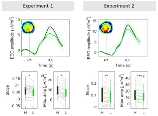
The reviewer is correct that properties such as temporal slope scaling with evidence strength and stereotyped threshold-like amplitude were key in establishing that the CPP reflects evidence accumulation in conventional continuous-stimulus tasks, and its motor independence was demonstrated in how it exhibited the same evidence-dependent dynamics in the absence of motor requirements (e.g. O'Connell et al 2012). We agree that it is of interest to check any such properties that can be feasibly tested in the current, distinct task context of intermittent evidence with delayed responses. Given the way in which participants performed our delayed-response task, sometimes terminating decisions early, it is in the CPP-P1 that conventional patterns of coherence-dependence in slope and amplitude would be expected. Indeed, we found that the CPP-P1 reached higher amplitudes (Fig. 3A, Author response image 1) and exhibited a steeper build up in high- compared to low-coherence trials (Author response image 1). The slope and amplitude profile of the CPP-P2 is complex due to the variability in baseline activity across our various delay conditions and the bounded process that participants engaged in, but it is still consistent with an accumulation process. Our simulations provide a full account of how an accumulating signal could produce the observed results.

Author response image 1.

Grand-averaged (± sem) CPP-P1 traces in both experiments (top). Bottom boxplot graphs indicate the average slope computed as the slope between 0.2 s post P1 onset (when CPP begins its buildup) and the time when peak amplitude was reached within the [0.4-0.6s] interval, computed for each subject individually. Red crosses indicate outliers, computed as values exceeding 1.5 times the interquartile range away from the bottom or top of the box. Grey lines indicate single subject estimates, and asterisks reflect the significance of paired ttests for the estimated slope and amplitude effects; **p<0.01, *p<0.05. H = high coherence, L = low coherence.

Like in other delayed-response tasks (Twomey et al 2016; McCone et al 2026), we observe here that the CPP peaks and falls well before the response is cued or indeed executed (here, in fact peaking and falling for each individual pulse). Thus, its pre-response dynamics will not relate to stimulus-driven evidence accumulation in the way they do in immediate response contexts (e.g. O’Connell et al. 2012; Steinemann et al. 2018). We therefore do not analyse response-aligned CPPs in the experiment.

As to the intermediary role we have interpreted for the CPP, in addition to the local pulse driven peak-and-fall dynamics compared to the sustained profiles of motor preparation signals, we can point to the obvious temporal delay between the signals, where evidence-dependent buildup in the CPP substantially precedes that of motor preparation, as observed in all previous studies comparing the two (e.g. Kelly & O'Connell 2013).

(2) The novelty of this work lies partly in the aim to characterize how the CPP and MBL interact (page 5, line 3-5). However, this analysis seems to be missing. E.g., at the single-trial level, do relatively strong CPP pulses predict faster/larger MBL? The simulations in Figure 5 are interesting, but more could be done with the measured physiology.

As exemplified in the extant EEG-decision literature, the low signal-to-noise ratio of EEG is such that attempts are seldom made to link two EEG signals on a single-trial basis, and studies instead favour testing single-trial relationships between each individual EEG signal and behaviour, or, most commonly, comparing patterns of variation in the EEG signals across experimental conditions (e.g. difficulty). Accordingly, here we show that trials with high coherence P1 evoked 1) higher CPP amplitudes (Fig. 3A,C), and 2) stronger MBL (Fig. S2 & S3). Further, we showed that particularly high CPP amplitudes following the first pulse led to stronger weights on choice for the first pulse (Fig. S11), which could only be mediated by the motor system.

(3) The focus on CPP and MBL is hypothesis-driven but also narrow. Since we know only a little about the physiology during this "gaps" task, have the authors considered computing TFRs from different sensor groupings (perhaps in a supplementary figure?).

While we agree that it might be interesting to explore frequency bands and sensors more broadly, we feel that such an exploration would detract from the hypothesis-driven focus on how prominent, well-characterised decision signals in the brain behave in a context where evidence is presented in an atypical, seldom-studied manner, namely in the form of temporally separate pulses. Our aim was not to explore whole-brain dynamics that might be engaged during the task, but rather to get a better understanding of the functional roles of the neural processes underlying the CPP and MBL during decision making. Providing a detailed description of whole-scalp responses is thus beyond the scope of this paper, but given that all data will be made publicly available this can be pursued in future work and by other researchers.

(4) The idea of a potential bound crossing during P1 is elegant, albeit a little simplistic. I wonder if the authors could more directly show a physiological signature of this. For example, by focusing on the MBL or occipital alpha split by the LL, LH, HL and HH conditions, and showing this pulse- as well as report-locked. Related, a primacy effect can also be achieved by modelling (i) self-excitation of the current one-dimensional accumulator, or (ii) two competing accumulators that produce winner-take-all dynamics. Is it possible to distinguish between these models, either with formal model comparison or with diagnostic physiological signatures?

In addition to the CPP amplitude effects we report in the main paper, the reviewer is correct that pulse-locked MBL can also provide a physiological signature of the greater number of pulse-1 bound crossings when that pulse is high-coherence. This is shown in Figure S3, where we see this coherence-dependent effect consistently across all gap durations and both experiments. Figure S2 also shows that the MBL step-change after P2 is greater in P1-low coherence trials in Experiment 1, as predicted by the bound-crossing account, and consistent with the CPP findings. We note that this effect appears absent in Experiment 2, but this is likely because the greater proportion of shorter gap durations (0, .12, .36s) mean that updates following P2 are likely to still capture P1-driven changes, due to signal-transmission delays. Please also note that Fig. S2 and S3 have been updated from the previous version, because while revising the paper we noticed a mistake whereby we were plotting alpha band power (813Hz) rather than the intended beta (13-30Hz). The results remain qualitatively unchanged. Although there isn’t sufficient single-trial signal-to-noise ratio to be able to categorise individual trials as having crossed a threshold or not, this is strong evidence in support of the coherence dependent amplitudes of the CPP and motor updates. Analyzing beta locked to the report would not be informative in this case because of the delayed reporting structure of the task and the threshold-crossing relationship beta exhibits with response execution (O’Connell et al. 2012). That is, beta will reach the same amplitude immediately prior to the response regardless of whether or not decisions were terminated during P1. Instead, we believe that the empirical CPP-P2 traces we show provide direct evidence that the second pulse was not fully integrated in all trials, and as our modelling confirms, this is consistent with bound crossings occurring sometimes before P2. First, the fact that CPP-P2 amplitudes were overall lower than CPP-P1 amplitudes mirrors the behavioural observation that the first pulse had a stronger weight on choice than the second one. Second, we show that trials where the CPP was particularly high after the first pulse were also trials where P1 also exerted a particularly strong influence on choice (see Fig. S11), further validating the idea that higher CPP amplitudes are directly related to behaviour.

Regarding self-excitation (SE) and winner-take-all competition (WTAC), these could indeed contribute to the behavioural primacy effects, but they would not detract from our central finding that the CPP does not encode a sustained representation of a decision variable, but rather reflects two rounds of evidence accumulation feeding into a single decision process. Further, it is not immediately clear whether/how these alternative models might also account for the CPP-P1/CPP-P2 results as simply as our bounded model does. While it might be theoretically possible for SE/WTAC models to explain 1) why the CPP-P2 is generally lower than the CPP-P1 across conditions, and 2) why the maximum CPP-P2 amplitudes in P1-high trials are smaller than in P1-low trials, these patterns of results are not an immediate consequence of standard implementations. Further, while the question of whether the accumulation process is perfect integration or involves SE or WTAC is certainly of additional interest, given that this is a delayed response task and does not provide information on termination timing through RT distributions, arbitrating between these modes of integration would not be straightforward with the current data.

(5) The way the authors specify the random effects of the structure of their mixed linear models should be specified in more detail. Now, they write: "Where possible, we included all main effects of interest as random effects to control for interindividual variability." This sounds as if they started with a model with a full random effect structure and dropped random components when the model would not converge. This might not be sufficiently principled, as random components could be dropped in many different orders and would affect the results. Do all main results hold when using classical random effects statistics on subject-wise regression coefficients?

The equations in the paper include the full details of the random effects structure we used for each model. We note that only two of our four equations did not include a full random effect structure, indeed due to convergence issues. We have now fit these models with a maximal random effects structure (i.e. including all fixed effects as random effects as well) with the ‘bobyqa’ optimiser. This resulted in singular fits for both Eq. 2 (Exp. 1 and Exp. 2) and Eq. 3 (Exp. 2 only). Following previous suggestions, we used a weakly informative wishart prior (Chung et al. 2015) to regularise the random effects covariance matrix using the blme package (Chung et al. 2013), which resolved the singular fit problem. However, the model still produced convergence warnings in some models. To assess these models’ robustness, we compared the fixed effect parameter estimates across multiple optimisers, as suggested by the lme4 developers (see lm4 documentation). Parameter estimates across optimisers rarely deviated by more than one decimal point across 6 optimisers (see Bates et al. 2011), and we thus concluded the model estimates were robust and convergence warnings were a false positive, a known issue in lme4. For all models in the paper, we report the parameters estimated using the “bobyqa” optimiser. All main inferential results remain unchanged (except for one interaction that was not of interest in Exp. 1), and the estimated slopes and statistical results for all models have been updated in the manuscript. We also included all these details in the manuscript.

Reviewer #2 (Public review):

Summary:

This manuscript examines decision-making in a context where the information for the decision is not continuous, but separated by a short temporal gap. The authors use a standard motion direction discrimination task over two discrete dot motion pulses (but unlike previous experiments, fill the gaps in evidence with 0-coherence random dot motion of differently coloured dots). Previous studies using this task (Kiani et al., 2013; Tohidi-Moghaddam et al., 2019; Azizi et al., 2021; 2023) or other discrete sample stimuli (Cheadle et al., 2014; Wyart et al., 2015; Golmohamadian et al., 2025) have shown decision-makers to integrate evidence from multiple samples (although with some flexible weighting on each sample). In this experiment, decision-makers tended not to use the second motion pulse for their decision. This allows the separation of neural signatures of momentary decision-evidence samples from the accumulated decision-evidence. In this context, classic electroencephalography signatures of accumulated decision-evidence (central-parietal positivity) are shown to reflect the momentary decision-evidence samples.

Strengths:

The authors present an excellent analysis of the data in support of their findings. In terms of proportion correct, participants show poorer performance than predicted if assuming both evidence samples were integrated perfectly. A regression analysis suggested a weaker weight on the second pulse, and in line with this, the authors show an effect of the order of pulse strength that is reversed compared to previous studies: A stronger second pulse resulted in worse performance than a stronger first pulse (this is in line with the visual condition reported in Golmohamadian et al., 2025). The authors also show smaller changes in electrophysiological signatures of decision-making (central parietal positivity and lateralised motor beta power) in response to the second pulse. The authors describe these findings with a computational model which allows for early decision-commitment, meaning the second pulse is ignored on the majority of trials. The model-predicted electrophysiological components describe the data well. In particular, this analysis of model-predicted electrophysiology is impressive in providing simple and clear predictions for understanding the data.

Weaknesses:

Some readers may be left questioning why behaviour in this experiment is so different from previous experiments, which use almost exactly the same design (Kiani et al., 2013; TohidiMoghaddam et al., 2019; Azizi et al., 2021; 2023). The authors suggest this may be due to the staircase procedure used to calibrate the coherence of (single-pulse) dot motion stimuli for individuals at the start of the experiment. But it remains unclear why overall performance in this experiment is so bad. Participants achieved ~85% correct following 400 ms of 33 - 45% coherent motion. In previous work, performance was ~90% correct following 240ms of 12.8% coherent motion. It seems odd that adding the 0% coherent motion in the temporal gaps would impair performance so greatly, given it was clearly colour-coded. There is a lack of detail about the stimulus presentation parameters to understand whether visual processing explains the declined performance, or if there is a more cognitive/motivational explanation.

We thank the reviewer for highlighting this. We apologise for not providing full details about the visual display, which we have included now.

The moving dots were presented centrally on the monitor, at a 5 degree aperture, and moving at a speed of 5 degrees/second. The monitor refresh rate was 60Hz for 19 participants and 85Hz for 3 participants in Experiment 1, while it was 85Hz for 19 participants and 60Hz for 2 participants in Experiment 2. Dot density in our task was similar to previous studies (16.7 dots/degree/s², as in Kiani & Shadlen 2013; Tohidi-Moghaddam et al. 2019; Azizi et al. 2021, 2023). However, in contrast to previous studies, we did not include any feedback on a trial-bytrial basis, instead only providing feedback at the end of each block indicating the average accuracy. This would have made it harder for participants to continually assess how well they were performing and to adjust their strategies (e.g. increase their bound for better accuracy) accordingly. We agree that the inclusion of 0% coherence dots during the gap between pulses is unlikely to have caused the participants’ relatively low overall performance, especially since we did not find accuracy to be overall lower for longer 0%-coherence gaps.

Further, as the reviewer notes, we used a staircasing procedure at the beginning of the experiment which used only single pulses of evidence. This may have encouraged participants to set a bound that can usually be reached by one pulse, and the resultant early terminations meant that they seldom used the full 400ms of evidence that were available to them. In fact, we would like to thank the reviewer for pointing out Golmohamadian et al., 2025, which used a similar variable delays task structure but with different visual stimuli. They, like us, trained on a single-pulse task version and omitted trial-by-trial feedback in the main task, and, also like us, reported a stronger choice reliance on pulse-1. This suggests that these two factors may suffice to induce a primacy rather than a recency effect.

There are other reasons why performance may have been different in our task compared to previous studies. For example, our task included a lead-in period that was longer than in previous studies and contained 0%-coherence dots, in order to minimise interfering VEP components (the lead in period was between 700 to 1050ms in our study, compared to 200– 500 ms in Kiani & Shadlen 2013; Tohidi-Moghaddam et al. 2019 & Azizi et al. 2023, and 400 -1000 ms in Azizi & Ebrahimpour 2021). This longer and visually explicit preparation period may have acted as a warning cue, allowing participants to fully prepare before the first pulse, and again making it easier for them to hit a bound with only that information.

We have added a more detailed discussion about how our stimuli and the task characteristics may have resulted in a substantially different performance in our task compared to previous studies in the discussion section.

Recommendations for the authors:

Reviewing Editor:

Please consider the following reviewer suggestions for how to strengthen the evidence for your central claims, which could translate into an improved assessment of the "strength of evidence".

Apart from these useful suggestions, I had some concerns about scholarship, because the list of studies currently cited in your introduction is exclusively from your group, while one of the phenomena of interest - motor beta power lateralization (MBL) in decision-making - has been widely studied by several groups, using also other techniques.

I was wondering why you chose not to cite the ample MEG evidence for the role of MBL in decision-making. This has been shown both in classical random dot motion tasks (Donner et al, Curr Biol, 2009; de Lange et al, J Neurosci, 2013; Pape et al, Nat Commun, 2016; Urai et al, Nat Commun, 2022) as well as in tasks involving discrete evidence samples (Wilming et al, Nat Commun, 2020; Murphy et al, Nat Neurosci, 2021). Another relevant EEG study is by Ian Gould et al, J Neurosci, 2010. There is also quite a bit of monkey LFP work (mainly by Saskia Haegens) on choice-selective beta power in the motor system of the macaque, although the link to the lateralized beta power suppression in your work and the above human E/MEG studies remains a bit elusive. I feel it would be important to provide a more balanced reflection of the existing literature on this phenomenon.

We thank the editor for this fair comment, and we apologise for having provided a too narrow, EEG-centric view of the literature, arising from our interest in the CPP component which hasn’t yet been characterised in MEG or LFPs. We have now substantially expanded the introduction to provide a more balanced and comprehensive overview of the literature.

Reviewer #1 (Recommendations for the authors):

(1) The diffusion model needs to be explained in more detail. For example, it should be explicitly stated that the model was fit to only choices, as most readers would expect reaction times. Further, it needs to be started if the model was fit separately for each subject or in one go to the group-level data. If the former, it is important to add error bars of the betweensubjects variability (in simulated and empirical data) to Figure 4A. If the latter, it would be important to determine uncertainty using bootstrapping.

The original model was fit to grand-average data, as stated in the methods section. To assess between-subjects variability, we have re-fitted the model to each individual subject, for each experiment. The average of the individually-estimated model parameters closely recapitulated the values obtained from the fit to grand-averaged data (Fig. S12). We then simulated N = 10000 trials for each individual, and we report the grand-averaged results with error bars indicating the standard error of the mean as a supplementary figure (Fig. S13). The results replicate the ones reported in the main manuscript. We have also made it explicit that the models are fit to accuracy data but not RT.

(2) The authors write numerous times that the MBL exhibits an "evidence-dependent" buildup. However, should this not be "choice-dependent"? In Figure 2A, one can clearly see that the sign of MBL follows choice and not objective evidence.

We thank the reviewer for this comment. By evidence-dependent, we mean that lateralisation towards the correct response is strongest in high-coherence trials (see Fig. S2, S3). This is indeed because the sign of MBL is choice-dependent, and participants are less likely to make mistakes in high-coherence trials. We have added a clarification sentence in the text.

(3) It would aid readability to add sub-conclusions at the end of each Results section.

We have added clarifications where needed.

(4) In Figure 1B, I cannot see a dashed line for the HL condition. I understand that it must lie under the LH condition, but it would be good to show it separately.

We thank the reviewer for this comment. Since we cannot show both lines separately without additional panels, given the HL and LH lines perfectly overlap, we indicate at the end of the caption that this is the case as follows: “Note that a perfect accumulator predicts identical accuracies for the HL and LH conditions, and therefore the two lines overlap.”

(5) In Figure 4B, is the horizontal dashed line important? It is confusing because the legend incorrectly states that this is "data".

Thanks for this observation - it was only there to indicate a 50% as a benchmark to assess how frequent early terminations are, but we agree that it was unnecessary and potentially confusing, so we have removed it from the plot.

Reviewer #2 (Recommendations for the authors):

(1) The authors should more directly address how behaviour in their task differs quite substantially from previous experiments with very similar designs (including why such high coherence levels are required, over a longer duration, to reach overall worse performance). Some readers may also be interested in a broader discussion of how decision-makers may use flexible weights when integrating evidence across samples over time. While the explanation of bounded accumulation is convincing in this context, Tsetsos et al., (2012) suggest recency effects (as in Cheadle et al., 2014; Wyart et al., 2015) cannot be explained by bounded accumulation, but rather integration leak. Other factors may include stimulus consistency (Glickman et al., 2022) or even choice consistency across decisions (Bronfman et all., 2015). Golmohamadian et al., 2025 demonstrated flexibility in decision strategies across sensory modalities.

As we described above, we have added some more detailed explanation about why it might be the case that behaviour in our study differs from previous reports using similar tasks. We agree that the reversed pulse-reliance in our study compared to others presents an opportunity to discuss flexibility in decision strategy and so we have now added a broader discussion on different patterns of integration in various task contexts. We thank the reviewer for pointing out Golmohamadian et al., 2025, as they, like us, trained on a single-pulse task version and omitted trial-by-trial feedback in the main task, and, like us, reported a stronger choice reliance on pulse-1.

(2) Another open question is how central parietal positivity reflects an accumulation signal in the case of continuous evidence, but reflects momentary evidence in the case of discrete evidence samples. If, in both cases, the parietal evidence is passed along to motor processes for bounded decision commitment, how do motor processes deal with the changes in what is represented? Can the relationship between MBL and CPP in the model-simulated data shed some light on this? Specifically, how is the 0-gap condition treated in this simulation (which shows only 1 CPP peak but with a longer time to decay) compared to non-zero gap conditions (which show 2 peaks)?

This is a very interesting and important point, and we thank the reviewer for raising it. We believe that the CPP in our intermittent-dots task reflects dot-motion evidence integration in the same way as in conventional continuous evidence tasks, building at an evidence dependent rate (see Author response image 1), with the only difference being that integration processes can be turned “on” or “off” depending on whether evidence is present, and can thus be temporally split into multiple “rounds” of accumulation when there is a gap.

Our model simulations assume that evidence integration is triggered by the dots turning yellow, indicating the presence of evidence, and feeds continuously to the motor system in these periods. However, it is switched off either when 1) a bound has been hit, or 2) the dots turn blue again, at which point the CPP falls (see various rates of signal decay in Fig. S7). The reason the CPP continues longer before it peaks and falls in the zero-gap condition, by this account, is because there is no dot-colour change at the end of pulse-1 to switch it off, and thus the accumulation process continues until either a bound is hit, or the yellow dots turn blue after pulse-2. When there is a non-zero gap, despite the CPP being switched off, the decision variable itself remains encoded at the motor level so that no information is lost. This requires that the same instruction that turns-off the CPP must also break or pause the flow from the CPP to the motor level and allow it to hold its current level until either a second pulse resumes a feed from a newly-triggered CPP, or response execution is cued. Thus, in our account, the accumulation process underlying the CPP in our intermittent-evidence task is identical to conventional continuous-evidence tasks, but since it can be turned “on” and “off” as a function of whether or not evidence is clearly present or absent, produces two “rounds” of integration in non-zero gap conditions. The motor process also receives a feed from the CPP as in conventional continuous-evidence tasks, but with this feed similarly gated by the presence of evidence.

A slightly different and perhaps more challenging question (which the reviewer was perhaps alluding to) relates to tasks where evidence comes not in short noisy snippets, but rather as static tokens (e.g. Wyart et al. 2012, 2015; Murphy et al. 2021; Parés-Pujolràs et al. 2025). In these instances, the CPP exhibits transient evoked responses to each token, which scale with the belief updates resulting from it (Parés-Pujolràs et al. 2025). However, it remains unclear whether these transient potentials reflect a temporally-evolving integration process to compute the appropriate belief update afforded by that token in the context of a particular task, or rather reflect the output of such a process. The former account would be similar to our interpretation of the transient deflections observed in this gaps task, which we believe capture the same temporal integration processes as those commonly observed in conventional continuous noisy stimuli paradigms, only short-lived. The latter account would instead be specific to low-noise stimuli like tokens, where the computations required for belief updating may not require a temporally-extended integration process, but rely on different mechanisms to compute belief updates (e.g. prior-based modulations of sensory encoding, attention or neural gain). These questions remain open for future investigation.

(3) From what I understand, the model suggests all-or-none integration of the second pulse: either the bound has not been reached and the pulse is perfectly integrated, or the bound has been reached and so the pulse is not integrated. The CPP amplitude at pulse 2 is therefore determined not only by the strength of the evidence at pulse 2 but also by the proportion of trials where the evidence is not ignored: CPP at pulse 2 is of lower amplitude because it is calculated as an average across trials where it is either similar to CPP at pulse 1 or otherwise completely absent. Another explanation for the lower average amplitude is that all trials have a smaller amplitude (somewhat different from the main conclusions of the paper). It would be nice to show the dichotomy predicted by the model in the empirical data. I'm thinking of something similar to this 'bifurcation' analysis from Sergent et al., 2021. Or more simply, estimates of CPP amplitude from single trials (perhaps an average over a short window around the peak) should be more variable at pulse 2, with some reaching similar amplitudes to pulse 1, and many close to baseline, whereas at pulse 1, there should be a more uniform cluster of amplitudes. If all CPP peak amplitudes were lower, would this motivate a model comparison where, for example, additional evidence from the second pulse was down-weighted according to certainty following the first pulse (leading to all trials down-weighting the second pulse)? This could link in nicely with some of the more nuanced analyses related to attention in the supplementary figures.

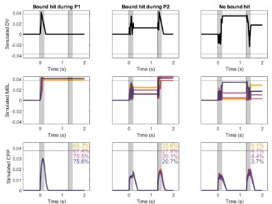
We thank the reviewer for this insightful comment, which will help us clarify how our model works. The integration of the second pulse does not work in an all-or-none manner. In our model, the accumulation stops whenever a bound is reached at the downstream motor level. This can happen 1) at some point during the 1st pulse (no integration of pulse 2 at all), 2) during the 2nd pulse (partial integration of pulse 2, until the bound is hit), or 3) not crossed at all (full integration of pulse 2). Our model thus allows for partial integration of the second pulse rather than all-or-none. Author response image 2 shows 3 example trials that illustrate how the model works. The CPP amplitudes at pulse 2 are thus determined by two main factors: 1) whether or not accumulation of P2 is precluded by an earlier bound crossing in P1 (if it is, the CPP amplitude is assumed to equal 0), and 2) whether and when accumulation ended if it did take place. Our interpretation is that, given that trials where pulse 1 was low coherence were 1) less likely to terminate early (Fig. 4B) and 2) had achieved lower levels of accumulated evidence (Fig. 4C), the LL and LH conditions are linked to a higher proportion of trials where accumulation at pulse 2 does occur, and it lasts for a longer amount of time because the distance required to reach a bound is longer than in their pulse 1 high-coherence counterparts. We have clarified this point in the results section describing the model.

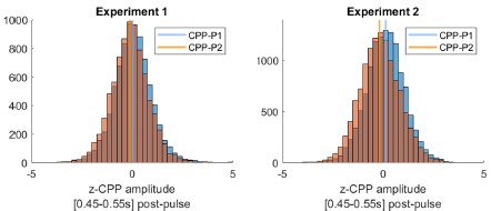
The reviewer notes: “Another explanation for the lower average amplitude is that all trials have a smaller amplitude (somewhat different from the main conclusions of the paper)”. However, our interpretation in fact predicts that the vast majority of trials should indeed exhibit smaller amplitudes. That can again be explained by the three trial types mentioned above. Unlike in CPP-P1, there would be a majority of trials where integration does not occur at all. Only trials where evidence was at least partially integrated during P2 would be predicted to have CPPP2 amplitudes that are overall positive, and even in those instances, average amplitudes would be overall lower than CPP-P1 in trials that terminated early, because of the lower distance remaining to be covered before hitting a bound. Author response image 2 illustrates this point. Thus, the prediction regarding how CPP amplitude variance or distribution shape would compare between P1 and P2 is less straightforward than if it were all-or-none on P2, not to mention the fact that EEG noise would likely drown-out distributional features like this. We therefore focus on a comparison of the means, for which our model has the clear prediction that most trials should exhibit lower CPP-P2 amplitudes. To assess whether empirical observations meet this prediction, and following the reviewer’s suggestion, we extracted the mean amplitudes around 0.45-0.55s after P1 and P2, for each single trial. CPP-P2 data were baselined using the amplitude 100 ms before P2 onset, as in Fig. S5 - note that this is likely to introduce spurious drifts due to overlapping potentials from P1, but given that grand averaged traces still qualitatively captured the key effects we assume it is a valid approach. We then pooled CPP-P1 and CPP-P2 amplitudes across pulses, and z-scored them for each participant separately. In both experiments, in a majority of participants (Exp. 1: 16/22, Exp. 2: 17/21) the median z-CPP-P1 amplitude was higher than that of z-CPP-P2. Author response image 3 illustrates the pooled distributions.

Author response image 2.

Decision variable simulations illustrating sample single trials (top) and CPP traces averaging data across conditions and N = 1000 trials (bottom), using model fits from Exp 2, in the long gap condition. Overlaid text indicates the percentage of trials in each subset, for each condition. The horizontal line indicates the bound; shaded areas indicate pulse presentation times. A. The bound was hit during P1, and therefore no further accumulation occurred during P2. B. The bound was hit during P2, and therefore P2 was only partially accumulated, C. No bound was hit, and therefore all evidence from P2 was accumulated.

Author response image 3.

Pooled CPP–P1 and CPP-P2 amplitudes [450-550ms post-pulse] distributions, normalised within-participant, and baselined 100ms before pulse onset. In both experiments, CPP-P2 amplitudes had a lower median (vertical line) normalised amplitude than CPP-P1.

(4) A minor note: Full details of stimulus presentation (size, number of dots, dot size, speed, lifetime) would be appreciated.

Thank you - we have now provided these details in the methods section (see also reply to public reviews above).

(5) Are the authors sure they want to use this 'Gaps task' name? It seems a bit strange to introduce this name in this context, where there isn't really a 'Gap' (random dot motion fills the gap). A reader could get the impression the name was given in the Kiani et al., 2013 study (page 3, paragraph 1: "This scenario has begun to be studied using an intermittent- evidence or "gaps" task (Kiani et al., 2013) ...") but this is not true, Kiani et al. never use the term "Gaps task", nor has any other study since (as far as I know).

We thank the reviewer for noting this oversight on our part - we have now made it clear that “gaps task” is the way we refer to the task originally developed by Kiani et al. 2013 in the introduction. We have decided to still use this name because it is a convenient proxy, in the understanding that “gap” refers to a “gap” in coherent motion as in Kiani et al (2013), albeit not a proper blank as in the original implementation.