Non-decision time-informed collapsing threshold diffusion model: A joint modeling framework with identifiable time-dependent parameters

Reviewer #1 (Public review):

Summary:

This paper proposes a non-decision time (NDT)-informed approach to estimating time-varying decision thresholds in diffusion models of decision making. The manuscript motivates the method well, outlines the identifiability issues it is intended to address, and evaluates it using simulations and two empirical datasets. The aim is clear, the scope is deliberately focused, and the manuscript is well written. The core idea is interesting, technically grounded, and a meaningful contribution to ongoing work on collapsing thresholds.

Strengths:

The manuscript is logically structured and easy to follow. The emphasis on parameter recovery is appropriate and appreciated. The finding that the exponential NDT-informed function produces substantially better recovery than the hyperbolic form is useful, given the importance placed on identifiability earlier in the paper. The threshold visualisations are also helpful for interpreting what the models are doing. Overall, the work offers a well-defined, methodologically oriented contribution that will interest researchers working on time-varying thresholds.

Weaknesses / Areas for Clarification:

A few points would benefit from additional clarification following the previous revision:

Returning to one point from my original review. The applications to empirical data describe 6 models, including the FT-DDM with across-trial variability described as a benchmark. Yet the modelling results for both studies (Tables 2 and 3) show only 5 models, omitting the benchmark model. I acknowledge the comment about this in the response letter (no other FT-DDM models in the main text have across-trial variability). Nevertheless, for this to serve as a benchmark, the modelling results really should be reported in Tables 2 and 3 with the other 5 models, and the model goodness of fit figures currently shown in Appendix 7 incorporated into Figures 10 and 13 of the main text. Unfortunately, as it currently reads, it looks as if something is being obscured, which I don't believe is the intention. This won't change the primary conclusions, but it will increase transparency and ease of interpretation.

Many thanks for introducing Appendix 1 to the revised manuscript. Additional motivation for the central issue is always helpful. However, I'm not (yet) convinced the simulation study in Appendix 1 achieves the intended aim. The simulation study shows that NDT misspecification leads to poorer recovery of other CT parameters (i.e., if a generating value is perturbed and then held fixed at that perturbed value during estimation, recovery of the remaining parameters deteriorates). This demonstrates the consequences of fixing NDT incorrectly, but it does not seem to address the central claim of the manuscript: that NDT and the CT threshold parameters trade off when they are estimated simultaneously. I had expected the simulation study to estimate NDT alongside the remaining model parameters, mirroring the estimation procedure used in the empirical analyses. Such a simulation would directly test whether the two sets of parameters compensate for one another during estimation, and whether this results in poor recovery of the NDT parameters.

Reviewer #2 (Public review):

Summary:

The authors use simulations and empirical data fitting in order to demonstrate that informing a decision model using noisy single-trial estimates of an underlying fixed non-decision time can guide the model to more reliable parameter estimates, especially when the model has collapsing bounds.

Strengths:

The paper is well written and motivated, with clear depth of knowledge in the areas of neurophysiology of decision-making, sequential sampling models, and in particular, the phenomenon of collapsing decision bounds.

Two large-scale simulations are run to test parameter recovery, and two empirical datasets are fit and assessed; the fitting procedures themselves are state-of-the-art, and the study makes use of a very new and well-designed ERP decomposition algorithm that provides single-trial estimates of the duration of diffusion; the results provide inferences about the operation of decision bound collapse - all of this is impressive.

Weaknesses:

This is an interesting and promising idea, but a very important issue is not clear: it is an intuitive principle that information from an external empirical source can enhance the reliability of parameter estimates for a given model, but how can the overall BIC improve, unless it is in fact a different model?

Comment on revised version.

Thanks to the authors for their responses and inclusion of additional analyses and simulations. Thanks, in particular for clarifying a crucial detail, that the ndt-informed model actually assumes, like the uninformed model, that there is no variability in the non-decision time, and the idea is that the variable single-trial measurements of non-decision time are noisy estimates of an underlying, constant ndt. The revised paper itself has not made this clear - for example, throughout the Intro, there is no statement that the behavioural model assumes a trial-invariant ndt, and line 231 still calls tau the 'mean' non decision time, implying there is a distribution rather than an invariant single value in the behavioural model.

One implication of the above is that if the lognormal sigma is purely measurement noise that does not relate to actual variation in the underlying decision process generating behaviour, then the HMP latencies should not relate to behaviour, e.g. shorter latencies predicting shorter RT. I assume that even if the authors did find such a relationship, the principle still stands that a model with fixed ndt is more accurately fit when there are single-trial ndt estimates whose mean provides a constraint on that ndt value, than without such measurements. Still, given ndt variability is a core feature of many decision models, the authors could comment on whether the strategy would work in theory for a model with ndt variability (in the behavioural part), where the single trial estimates would then presumably reflect a mix of measurement noise and genuine ndt variability.

Another more important implication is that since it is in fact the same model being compared with and without the HMP data guiding the fixed ndt estimate, the reason the fit quality improves with HMP-information is not because it is a better model per se (it is the same model) but because without the HMP guidance, the search algorithm somehow gets lost and fails to find the 'optimal' parameter vector. That is, the parameter vector (just the parameters that relate to the behavioural model itself, not the HMP lognormally-distributed noise associated with VEP measurements) identified as optimal in the HMP-informed version of the model exists in the parameter space of the model without HMP information, but it is just not found? I raised this implication before, and it is still not clear whether it applies. I'm sorry to press on it, but it is critical for readers to understand why it is that neural information can improve overall model fit. Again, the enhancement of parameter recovery (like in Nunez 2025) makes sense, but the enhancement of the "model's fit to behavioural data" does not, without pointing to a deficiency in the search algorithm / fitting procedure.

The authors state in their replies that the onset of bound collapse is set at accumulation onset and imply that setting it instead at stimulus onset could "mathematically resolve the issue" but they don't do it because it is implausible. It is in fact not only plausible but clearly evidenced in empirical data - collapsing bounds are implemented neurally through urgency signals, and these can begin to dynamically build toward threshold well before, let alone at, stimulus onset. There is nothing bizarre about this - we can prepare movements without sensory input, and indeed even if choosing actions based on a sensory discrimination, motor preparation can launch well before the sensory evidence (e.g. Stanford, Salinas et al 2010) and this in effect collapses the bound on cumulative evidence for triggering action before any evidence actually arrives. So, Urgency/bound-collapse does not need to be triggered by a stimulus; it can start in anticipation of the stimulus. It seems critical, therefore, for the authors to clarify this point - does re-defining the onset of the collapse at stimulus onset remove the trade-off and render unnecessary the neurally-informed ndt estimation?

Related to this, it is still not clear how bias in the estimation of nondecision time would not be a problem. What if, for example, it is the end of the N2 rather than the peak of the N2 that marks accumulation onset, and/or there is an additional fixed motor time that adds to the N2-based marker to make the full nondecision time that applies in the underlying decision process. By definition (and I think this is essentially what the authors' new simulations verify), because of the trade-offs, this bias would simply be absorbed in shifted estimates of theta and lambda describing the bound collapse function. But wasn't the whole point of the exercise to more accurately estimate those parameters? The obvious implication is that the parameter-estimation accuracy of the ERP-informed model is determined by the accuracy with which the proposed ERP marker directly pinpoints the full nondecision time without bias, but this is not at all obvious in the paper as written. Importantly, in the example scenario I describe above where accumulation onsets when N2 ends, there may still be a perfect correlation of N2 peak latency with underlying ndt across trials - they could still be very strongly "linked" statistically, but we can't know what size offset might be involved.

Reviewer #3 (Public review):

The current paper addresses an important issue in evidence accumulation models: many modelers implement flat decision boundaries because the collapsing alternatives are hard to reliably estimate. Here, using simulations the authors demonstrate that parameter recovery can be drastically improved by providing the model with additional data (specifically, an EEG-informed estimate of non-decision time). Moreover, in two empirical datasets it is shown that those EEG-informed models provide a better fit to the data. The method seems sound and promising and might inform future work on the debate regarding flat vs collapsing choice boundaries. As an evidence-accumulation enthusiast, I am quite excited about this work, although for the more broader audience the immediate applicability of this approach seems limited because it does require EEG data (i.e. limiting widespread use of the method or e.g. answering questions about individual differences that require very large N).

Comments on revised version.

I thought the authors carefully addressed my concerns.

Author response:

The following is the authors’ response to the original reviews.

Reviewer #1 (Public review):

Summary:

This paper proposes a non-decision time (NDT)-informed approach to estimating timevarying decision thresholds in diffusion models of decision making. The manuscript motivates the method well, outlines the identifiability issues it is intended to address, and evaluates it using simulations and two empirical datasets. The aim is clear, the scope is deliberately focused, and the manuscript is well written. The core idea is interesting, technically grounded, and a meaningful contribution to ongoing work on collapsing thresholds.

Strengths:

The manuscript is logically structured and easy to follow. The emphasis on parameter recovery is appropriate and appreciated. The finding that the exponential NDT-informed function produces substantially better recovery than the hyperbolic form is useful, given the importance placed on identifiability earlier in the paper. The threshold visualisations are also helpful for interpreting what the models are doing. Overall, the work offers a well-defined, methodologically oriented contribution that will interest researchers working on time-varying thresholds.

We appreciate the positive and constructive feedback. We have addressed your comments in the revised manuscript, as detailed in our responses to the specific comments below.

Weaknesses / Areas for Clarification:

A few points would benefit from clarification, additional analysis, or revised presentation:

(1) It would help readers to see a concrete demonstration of the trade-off between NDT and collapsing thresholds, to give a sense of the scale of the identifiability problem motivating the work.

Thank you for this constructive suggestion. We conducted a new simulation study in which we considered the non-decision time as a fixed parameter and estimated the remaining parameters of the collapsing threshold model. In this simulation study, we contaminated the non-decision time with noise at six levels (i.e., 0%, 2%, 4%, 6%, 8%, and 10%). The simulation results showed that increasing the noise level in non-decision time worsens the estimation of the starting threshold and decay rate parameters, indicating a trade-off between non-decision time and collapsing threshold parameters. The results of this simulation are presented in Appendix 1 in the new version of the manuscript.

(2) Before moving to the empirical datasets, the manuscript really needs a simulation-based model recovery comparison, since all major conclusions of the empirical applications rely on model comparison. One approach might be to simulate from (a) an FT model with across-trial drift variability and (b) one of the CT models, then fit both models to each of the simulated data sets. This would address a longstanding issue: sometimes CT models are preferred even when the estimated collapse in the thresholds is close to zero. A recovery study would confirm that model selection behaves sensibly in the new framework.

We are grateful for this constructive comment. The revised manuscript includes a model recovery study (see Simulation study 2, in particular Table 1 and the accompanying text). In this simulation, as the reviewer suggested, we generated data from FT-DDM with across-trial variability in drift rate and CT-DDM with hyperbolic and exponential collapsing thresholds. Then, for each generated dataset, we fitted two models and classified the datasets based on goodness-of-fit and estimated decay rate. The results show that incorporating the decay rate, which can be reliably estimated by the NDT-informed modeling framework, significantly improves the precision of model recovery.

(3) An additional subtle point is that BIC is defined in terms of the maximised log-likelihood of the model for the data being modelled. In the joint model, the parameter estimates maximise the combined likelihood of behavioural and non-decision-time data. This means the behavioural log-likelihood evaluated at the joint MLEs is not the behavioural MLE. If BIC is being computed for the behavioural data only, this breaks the assumptions underlying BIC. The only valid BIC here would be one defined for the joint model using the joint likelihood.

We thank the reviewer for raising this important methodological point. We agree that, strictly speaking, the behavioral log-likelihood evaluated at the joint maximum likelihood estimates is not guaranteed to be equal to the behavioral maximum likelihood estimate. Therefore, if one were to interpret BIC_Behavior for joint (NDT-informed) models as a conventional BIC derived from a purely behavioral maximum likelihood fit, this would indeed violate the standard assumptions underlying BIC. Our intention, however, was not to claim that BIC_Behavior represents a formally valid BIC in the strict information-theoretic sense. Rather, we used it as a diagnostic measure to assess how well the jointly estimated parameters account for the behavioral data relative to the uninformed models. Importantly, in our datasets, the behavioral log-likelihood evaluated at the joint estimates is higher than that obtained from the uninformed models. This suggests that the additional constraint introduced by the non-decision time information helps guide the optimization procedure toward parameter regions that provide a better account of the behavioral data. In other words, uninformed models appear to converge to suboptimal parameter estimates, but the joint modeling framework helps regularize the estimation process and yields better estimates of the optimal parameters. We fully acknowledge that this use of BIC_Behavior for the joint models departs from standard practice in the cognitive modeling literature. For this reason, we rely primarily on the joint likelihood–based model comparison as the formally valid criterion. The behavioral BIC is reported only to provide additional intuition regarding the goodness of fit on behavioral data and is used exclusively to compare NDT-informed models with their uninformed counterparts under identical evaluation criteria.

Also, to warn readers about this limitation, we included the following statement in the section where we defined BIC measures:

“It is worth noting that comparing joint and behavioral models using BIC_Behavior is uncommon and constitutes a limitation of the model comparison study.”

(4) Table 1 sets up the Study 1 comparisons, but there’s no row for the FT model. Similarly, Figures 10 and 13 would be more informative if they included FT predictions. This matters because, in Study 1, the FT model appears to fit aggregate accuracy better than the BIC-preferred collapsing model, currently shown only in Appendix 5. Some discussion of why would strengthen the argument.

In the revised manuscript, we have included the results for NDT-informed FT-DDM in the main text. However, we kept the FT-DDM with drift variability in the appendix, since none of the models in the main text include drift rate variability.

(5) In Figure 7, the degree of decay underestimation is obscured by using a density plot rather than a scatterplot, consistent with the other panels of the same figure. Presenting it the same way would make the mis-recovery more transparent. The accompanying text may also need clarification: when data are generated from an FT model with across-trial drift variability, the NDT-informed model seems to infer FT boundaries essentially. If that’s correct, the model must be misfitting the simulated data. This is actually a useful result as it suggests across-trial drift variability in FT models is discriminable from collapsing-threshold models. It would be good to make this explicit.

Regarding the visualization of decay rate estimation in Figure 7, we would like to clarify that, in the data-generating process for the FT model with across-trial drift variability, the decay rate is fixed at zero. That is, unlike the other parameters, there is only a single true value on the x-axis. If we were to present the decay rate recovery using a standard scatter plot (true vs. estimated values), all points would lie vertically above the single true value (zero), resulting in a vertical strip of points. While such a plot would technically be consistent with the other panels, it would not clearly convey the distributional properties of the estimated decay rates, specifically, which values are more likely under model misidentification. For this reason, we chose a density plot to more transparently illustrate the distribution of inferred decay rates when the true generating process is an FT model. We believe this representation more effectively communicates the extent and structure of mis-recovery. To avoid confusion, we have added a clarifying footnote in the revised manuscript explaining why a density plot was used in this specific panel.

Regarding distinguishing fixed-threshold models from collapsing-threshold models, as suggested in your comment 2, we conducted an additional simulation, and the results showed that when using the NDT-informed diffusion model, we can distinguish between both models with high accuracy. Specifically, we showed that incorporating the estimated decay rate value provided by the NDT-informed modeling approach can significantly improve the model recovery accuracy.

(6) Given the large recovery advantage of the exponential NDT-informed function over the hyperbolic one, the authors may want to consider whether the results favour adopting the former more generally. Given these findings, I would consider recommending the exponential NDT-informed model for future use.

Consistent with the reviewer’s argument, we included the following text in the general discussion:

“Importantly, the exponential collapsing threshold exhibited substantially better parameter recovery and superior model recovery performance, suggesting that this specification may be preferable in future cognitive modeling applications.”

(7) In Study 2 (Figure 13), all models qualitatively miss an interesting empirical pattern: under speed emphasis, errors are faster than corrects, while under accuracy emphasis, errors become slower. The error RT distribution in the speed condition is especially poorly captured. It would be helpful for the authors to comment, as it suggests that something theoretically relevant is missing from all models tested.

Thank you for mentioning this point. Because the models considered in the main text do not include across-trial variability in the starting point, the model cannot predict the fast error pattern observed in the speed condition of the second study. In the revised manuscript, we included a note on this point:

“The NDT-informed models’ predictions are depicted in Figure 13. This figure shows that the FT-DDM overestimates the last RT quantiles for both correct and incorrect responses in both speed and accuracy conditions. However, the qualitative predictions of CT-DDMs align more closely with the empirical data. It is also worth noting that all the considered computational models misfit the incorrect responses in the speed condition. This misfit is to be linked to the presence of fast errors, specifically in the speed condition. Including the starting-point variability parameter in the model enables the model to predict fast errors. However, as the aim here was not merely to fit the data with the best possible model, but to test the NDT-informed modeling framework, we did not include starting-point variability in the model.”

(8) The threshold visualisations extend to 3 seconds, yet both datasets show decisions mostly finishing by 1.5 seconds. Shortening the x-axis would better reflect the empirical RT distributions and avoid unintentionally overstating the timescale of the empirical decision processes.

In the new version of the manuscript, we shortened the x-axis in these plots. See Figures 9 and 12 in the new version of the manuscript.

Reviewer #1 (Recommendations for the authors):

(1) The manuscript should explicitly state how critical the log-normal assumption for NDT is, and whether there are caveats if it doesn’t hold.

We agree with this suggestion. Therefore, we conducted an additional simulation study in which we assumed a normal distribution for non-decision time measurements and replicated the main results reported in simulation study 1 (see Appendix 8 in the new version of the manuscript). These simulation results reveal that independent of distributional assumptions on non-decision time measurements, constraining non-decision time can improve the estimation of the collapsing threshold.

(2) On page 14, one paragraph refers to five models and another to six. It is unclear which is correct.

We are sorry for the confusion. In the new version of the manuscript, we addressed this issue.

(3) In the Discussion: Hawkins & Heathcote (2021) found that NDT estimates in the TRDM recover well, but the timer-offset parameter does not (and hence is set to a fixed value). It would be interesting to test whether the NDT-informed approach could extend to that parameter. The TRDM can also generate error RT distributions that are faster than correct RT distributions, which is the qualitative pattern that none of the present models capture in the speed condition of Study 2.

We appreciate the reviewer’s suggestion, as it would be another important demonstration of the framework we built in the paper. Nevertheless, given the number of models already considered in the manuscript and the focus on collapsing threshold diffusion models, we believe that this addition would blur the focus of the present manuscript. Therefore, we have decided not to include TRDM in the manuscript. Nevertheless, we have addressed the reviewer’s concern regarding the non-decision time estimation in the TRDM in the revised manuscript:

“Notably, this model can also predict faster error responses than the correct response, the pattern that is observed in the speed condition of Study 2. However, the authors reported poor parameter recovery for the onset of the timing process (Hawkins and Heathcote, 2021). Thus, the reliability issue here specifically concerns the estimation of the shift parameter of the timing accumulator. Informing the model with external estimates of non-decision time might, therefore, improve parameter recovery in this model as well.”

Reviewer #2 (Public review):

Summary:

The authors use simulations and empirical data fitting in order to demonstrate that informing a decision model on estimates of single-trial non-decision time can guide the model to more reliable parameter estimates, especially when the model has collapsing bounds.

Strengths:

The paper is well written and motivated, with clear depth of knowledge in the areas of neurophysiology of decision-making, sequential sampling models, and, in particular, the phenomenon of collapsing decision bounds.

Two large-scale simulations are run to test parameter recovery, and two empirical datasets are fit and assessed; the fitting procedures themselves are state-of-the-art, and the study makes use of a very new and well-designed ERP decomposition algorithm that provides single-trial estimates of the duration of diffusion; the results provide inferences about the operation of decision bound collapse - all of this is impressive.

We appreciate your feedback and comments. Below, we provided a response for each comment.

Weaknesses:

(1) This is an interesting and promising idea, but a very important issue is not clear: it is an intuitive principle that information from an external empirical source can enhance the reliability of parameter estimates for a given model, but how can the overall BIC improve, unless it is in fact a different model? Unfortunately, it is not clear whether and how the model structure itself differs between the NDTinformed and non-NDT-informed cases. Ideally, they are the same actual model, but with one getting extra guidance on where to place the tau and/or sigma parameters from external measurements. The absence of sigma (non-decision time variance) estimates for the non-NDT-informed model, however, suggests it is different in structure, not just in its lack of constraints. If they were the same model, whether they do or do not possess non-decision time variability (which is not currently clear), the only possible reason that the NDT-informed model could achieve better BIC is because the non-NDT-informed model gets lost in the fitting procedure and fails to find the global optimum. If they are in fact different models - for example, if the NDT-informed model is endowed with NDT variability, while the non-NDT-informed model is not - then the fit superiority doesn’t necessarily say anything about an NDT-informed reliability boost, but rather just that a model with NDT variability fits better than one without.

To respond to this comment, we would like to note that the structural difference between NDT-informed and uninformed models is the assumption about non-decision time. In principle, the behavioral parts (i.e., parameters related to the diffusion part) of both NDT-informed and uninformed models are identical. However, during the estimation, the non-decision time in the NDT-informed model is subject to an additional constraint imposed by the neural data. In other words, in the uninformed model, non-decision time is estimated using the behavioral data by maximizing the likelihood of a CT-DDM. However, the NDT-informed model incorporates an additional data type, resulting in a different likelihood function (see Equation (3)). Specifically, in the NDT-informed model, we make an additional assumption regarding the non-decision time: it is set to the mean of the trial-level non-decision time measurements distribution derived from neural data (Equation (3) specifies the joint model structure). This additional assumption constrains the search space of the non-decision time parameter in the NDT-informed model. As in the main text, we assumed that non-decision time measurements obtained from neural data are log-normally distributed, where sigma is the shape parameter of the log-normal distribution. Therefore, sigma can represent the variability of the non-decision time measurements, and it is not the trial-to-trial non-decision time variability parameter. Indeed, the non-decision time parameter is fixed across trials in both models. Also, it should be clear from Equation (3) that sigma only appears in the second term of the joint likelihood, which corresponds to non-decision time measurements and not the CT-DDM term. Therefore, the behavioral parts of the NDT-informed models and Uninformed models are identical, and the NDT-informed models include one additional parameter (i.e., sigma) corresponding to the variability in non-decision time measurements.

Also, to explain how constraining non-decision time improves the BIC, we would like to clarify that constraining non-decision time using an additional data source constrains the search space for non-decision time, thereby leading to better parameter identification and, consequently, a better fit to behavioral data. We included the following text in the discussion section to make this explicit.

“This improvement likely reflects more accurate parameter estimation enabled by the additional information. In other words, constraining the non-decision time using neural measurements led the optimizer to estimate the CT-DDM parameter more accurately and, as a result, improve the fit to empirical data.”

(2) One reason this is unclear is that Footnote 4 says that this study did not allow trial-to-trial variability in nondecision time, but the entire premise of using variable external single-trial estimates of nondecision times (illustrated in Figure 2) assumes there is nondecision time variability and that we have access to its distribution.

We are sorry for the confusion. To respond to this comment, we would like to highlight that this modelling approach does not include any mechanism for across-trial variability in the behavioral part, as the likelihood of the choice behavior (see Equation (3)) does not include any variability parameter. As mentioned before, sigma represents the variability in non-decision measurements. However, the model does not propagate the across-trial variability of the neural data on the behavior side (unlike the models in Ghaderi-Kangavari et al. 2023). In other words, in this approach, none of the diffusion model’s parameters include across-trial variability, and we have only considered and estimated neural data variability in the NDT-informed model. Also, to improve the manuscript’s coherence, we removed this footnote.

(3) It is good that there is an Intro section to explain how the tradeoff between NDT and collapsing bound parameters renders them difficult to simultaneously identify, but I think it needs more work to make it clear. First of all, it is not impossible to identify both, in the same way as, say, pre- and postdecisional nondecision time components cannot be resolved from behaviour alone - the intro had already talked about how collapsing bounds impact RT distribution shapes in specific ways, and obviously mean (or invariant) NDT can’t do that - it can only translate the whole distribution earlier/later on the time axis. This is at odds with the phrasing “one CANNOT estimate these three parameters simultaneously.” So it should be first clarified that this tradeoff is not absolute. Second, many readers will wonder if it is simply a matter of characterising the bound collapse time course as beginning at accumulation onset, instead of stimulus offset - does that not sidestep the issue? Third, assuming the above can be explained, and there is a reason to keep the collapse function aligned to stimulus onset, could the tradeoff be illustrated by picking two distinct sets of parameter values for non-decision time, starting threshold, and decay rate, which produce almost identical bound dynamics as a function of RT? It is not going to work for most readers to simply give the formula on line 211 and say ”There is a tradeoff.” Most readers will need more hand-holding.

We are grateful for this comment. In response to this comment, which was also partly mentioned by the first reviewer, we first highlight that, in the presence of a nonlinear collapsing threshold, the effect of non-decision time is no longer linear, as it forces the threshold to take a specific value at the final stopping point. To illustrate the tradeoff between imprecise non-decision time estimation and collapsing threshold estimation, we conducted a simulation study. The results for the simulation study are presented in Appendix 1. In this study, we contaminated the non-decision time with noise at six levels (i.e., 0%,2%,4%,6%,8%, and 10%). The simulation results showed that increasing the noise level in non-decision time worsens the estimation of the starting threshold and decay rate parameters, indicating a trade-off between non-decision time and collapsing threshold parameters.

Regarding the second point, we would like to clarify that in this paper, consistent with other works on collapsing threshold, we assumed that the collapsing starts with evidence accumulation and not with stimulus onset, as the decision makers need a short amount of time for perceiving and encoding the stimulus (i.e., perceptual encoding time). Fixing the collapsing onset to the stimulus onset introduces an ad hoc assumption into the model (that the encoding time is zero), which is cognitively implausible. Therefore, although this assumption can mathematically resolve the issue, it is not cognitively plausible. However, one important point we did not consider in the previous version is the two-stage accumulation process models in which the collapsing onset occurs later than the evidence-accumulation onset. We have discussed the estimation of such models as a limitation in the general discussion:

“The collapsing threshold dynamics considered in this work (e.g., exponential and hyperbolic) impose a monotonically decreasing threshold over time. Although these dynamics are theoretically well motivated (Fudenberg et al., 2018; Frazier and Yu, 2007) and have been employed in several previous studies (e.g., Olschewski et al., 2025; Milosavljevic et al., 2010; Voskuilen et al., 2016), some research has proposed delayed-collapsing threshold models (e.g., Diederich and Oswald, 2016), in which the onset of threshold collapse does not coincide with the onset of evidence accumulation. Estimating such delayed-collapsing models may require more than simply constraining non-decision time, as the onset of threshold collapse must also be identified. A promising approach for addressing this challenge is the HMP method, which may provide additional temporal information about distinct cognitive processing stages. In particular, HMP may allow the onset of threshold collapse to be estimated as a separate cognitive stage. Future research should therefore investigate the estimation of multi-stage evidence accumulation models (e.g., Diederich and Oswald, 2016; Diederich and Colonius, 2021) within the HMP framework.”

(4) A lognormal distribution is used as line 231 says it “must” produce a right-skew. Why? It is unusual for non-decision time distribution to be asymmetric in diffusion modeling, so this “must” statement must be fully explained and justified. Would I be right in saying that if either fixed or symmetrically distributed nondecision times were assumed, as in the majority of diffusion models, then the non-identifiability problem goes away? If the issue is one faced only by a special class of DDMs with lognormal NDT, this should be stated upfront.

We would like to clarify that this assumption is about the non-decision time measurements and not about the across-trial variability parameter of non-decision time. Although for computational convenience, non-decision time is often assumed to follow a normal distribution in diffusion modelling literature, some empirical studies have shown that the perceptual encoding time and total approximated non-decision time follow a right-skewed distribution. Moreover, as HMP estimations of non-decision time are usually right-skewed, we formalized the model with a log-normal distribution. However, we would like to note that the identifiability issue in collapsing-threshold diffusion models is not related to the distributional assumption over the non-decision time measurements, as poor parameter recovery of the collapsing threshold was also reported in Evans et al. (2020). To show that the distributional assumption about the non-decision time measurements does not affect the results, we conducted an additional simulation study in which we assumed a normal distribution for non-decision time measurements and showed that constraining non-decision time improves parameter recovery for collapsing threshold parameters. The results for this simulation are presented in Appendix 8 in the new version of the manuscript. We also revised line 231 as follows (see line 236 in the new version):

“Empirical studies on non-decision time measurement usually have reported a right-skewed distribution for their measurements (e.g., Weindel, 2021; Weindel et al., 2025). For instance, the measured perceptual encoding time and motor execution time reported by Weindel et al. (2025) are right-skewed. Therefore, we assume that the observed non-decision time measurements Z_n follow an approximate log-normal distribution, which is right-skewed (we will discuss how this distributional assumption can affect the results later). Thus, we model the non-decision time measurements Z_n, using a log-normal distribution with parameters µ and σ_z. The available measurements (i.e., observed data) at trial n can be represented as

follows:”

(5) In the simulation study methods, is the only difference between NDT-informed and non-informed models that the non-NDT-informed must also estimate tau and sigma, whereas the NDT-informed model “knows” these two parameters and so only has the other three to estimate? And is it the exact same data that the two models are fit to, in each of the simulation runs? Why is sigma missing from the uninformed part of Figure 4? If it is nondecision time variability, shouldn’t the model at least be aware of the existence of sigma and try to estimate it, in order for this to be a meaningful comparison?

As mentioned in the response to your first comment, the difference between NDT-informed and uninformed models is the access to an additional source of data related to non-decision time, and sigma represents the shape parameter of the non-decision time measurements distribution. Therefore, sigma belongs only to the NDT-informed model, and, as in the uninformed model, there is no additional data source, so the model does not include sigma.

(6) I am curious to know whether a linear bound collapse suffers from the same identifiability issues with NDT, or was it not considered here because it is so suboptimal next to the hyperbolic/exponential?

Thank you very much for this comment. The main reason we did not include linear collapsing threshold models was the assessment by Evans et al. (2020), which indicated that, with sufficient trials, these models can be estimated reasonably well. However, to investigate whether constraining non-decision time can also improve the estimation of linear collapsing threshold models, we conducted an additional simulation study, which is reported in Appendix 3 in the new version of the manuscript. The simulation results confirm those reported by Evans et al. (2020) and show that the parameters of the uninformed linear models can be identified using more than 500 trials. Constraining the non-decision time using the NDT-informed diffusion modeling framework still improves parameter estimation in the linear collapsing threshold model and reduces the required number of trials for reliable estimation to 250. Especially, the estimation of the starting threshold improves significantly.

(7) The approach using HMP rests on the assumption that accumulation onset is marked by the peak of a certain neural event, but even if it is highly predictive of accumulation onset, depending on what it reflects, it could come systematically earlier or later than the actual accumulation onset. Could the authors comment on what implications this might have for the approach?

Thank you for mentioning this point. We first would like to point out that Weindel et al. (2024) showed that HMP can predict the underlying generative distribution of cognitive states with high precision and without systematic bias. Second, it is worth highlighting the results reported in Appendix 5 (i.e., “Bias in non-decision time measurements”). In this appendix, we discussed how bias in non-decision time measurements (i.e., systematic underestimation or overestimation) affects the estimation of the collapsing threshold. Particularly, see Figure 3 in Appendix 5. To make these results clearer in the main text, we included the following paragraph at the end of the results section in simulation study 1:

“Additionally, we examined the effect of systematic bias in non-decision time measurement on parameter recovery. Appendix 5 presents the parameter recovery simulation results in the presence of biased non-decision time measurement (i.e., systematically underestimated or overestimated). The results revealed that, even in the presence of biased non-decision time measurement, the actual generating parameters show a high correlation with the estimated parameters. Underestimation in non-decision time leads to overestimation in the starting threshold and decay rate. Conversely, overestimation in non-decision time leads to underestimation in both the starting threshold and non-decision time.”

(8) Figure 7: for this simulation, it would be helpful to know the degree to which you can get away with not equipping the model to capture drift rate variability, when the degree of that d.r. variability actually produces appreciable slow error rates. The approach here is to sample uniformly from ranges of the parameters, but how many of these produce data that can be reasonably recognised as similar to human behaviour on typical perceptual decision tasks? The authors point out that only 5% of fits estimate an appreciable bound collapse but if there are only 10% of the parameter vectors that produce data in a typical RT range with typical error rates etc, and half of these produce an appreciable downturn in accuracy for slower RT, and all of the latter represent that 5%, then that’s quite a different story. An easy fix would be to plot estimated decay as a scatter plot against the rate of decline of accuracy from the median RT to the slowest RT, to visualise the degree to which slow errors can be absorbed by the no-dr-var model without falsely estimating steep bound collapse. In general, I’m not so sure of the value of this section, since, in principle, there is no getting around the fact that if what is in truth a drift-variability source of slow errors is fit with a model that can only capture it with a collapsing bound, it will estimate a collapsing bound, or just fail to capture those slow errors.

Thank you for this comment. We would like to first note that the aim of this section is to illustrate that NDT-informed modeling enables us to distinguish between CT-DDM and FT-DDM with drift variability (i.e., the two competing models that are relatively hard to distinguish). Therefore, we changed the name of this section to “Simulation study 2: Model recovery”. In the new version of the manuscript, we included a cross-model fitting simulation and a model recovery simulation in this section. The estimated decay rates in the cross-model fitting study indicate that, when the underlying generating model is FT-DDM with drift variability, parameter estimation using the NDT-informed approach yields precise inference. This is due to the estimated decay rate, which is very close to zero. The model recovery results also confirmed that incorporating the decay rate value into the model inference improves precision.

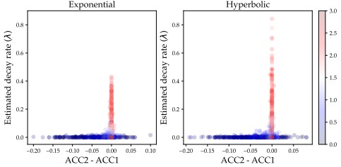
Moreover, to address the concern regarding the slow-error pattern in the simulated data, we examined the relationship between the slow–fast accuracy difference and the estimated decay rate. Specifically, we computed the difference between the accuracy of responses with response times below the median (ACC1) and those above the median (ACC2), and plotted this difference against the estimated decay rate. Author response image 1 presents the resulting scatter plot, with color indicating the drift rate. As shown in Author response image 1, incorrect inferences about the decay rate primarily occur at high drift rates. This pattern emerges because high drift rates produce very fast responses, leaving little time for the threshold to meaningfully collapse. Consequently, the behavioral signatures of collapsing-threshold and fixed-threshold models become increasingly similar under high drift conditions.

Author response image 1.

Illustration of the difference between the accuracies of responses with response time below the median and those with response time above the median against the estimated decay rate. Colour shows the drift rate value.

Reviewer #2 (Recommendations for the authors):

(1) Abstract: improves fit to behaviour in what way? Reliability or absolute quant fit to behavior? I.e., is it just helping constrain it so it finds the global opt?

(2) Line 72 - Are these “neuroimaging” studies? Perhaps use the broader term “neuroscience.”

(3) Line 95 - It’s important because it may confuse readers how something dynamic like a collapsing bound could be resolved with, say, fMRI.

(4) Line 85 – “greater variability”... in what?

(5) Line 87 -Revise to avoid misconstruing a time on task effect - e.g., “higher error rate for trials with longer RT” is more explicit.

(6) Line 89-94 - It’s not clear what findings are being referenced here.

(7) Line 103 - External biases such as priors and relative value?

(8) Line 175 - Clarify this applies to any ddm, not just ctddm.

(9) Line 268 - Explain what portion N200 accounts for.

(10) Line 327 - Is this equation supposed to be for Delta-X, as opposed to X(t+delta-t)? If you want X(t+delta-t) on the LHS, then X(t) must be added to the RHS.

We are very thankful for such a precise evaluation and constructive comments. We addressed all the comments raised by the reviewer in the revised manuscript.

Reviewer #3 (Public review):

Summary:

The current paper addresses an important issue in evidence accumulation models: many modelers implement flat decision boundaries because the collapsing alternatives are hard to reliably estimate. Here, using simulations, the authors demonstrate that parameter recovery can be drastically improved by providing the model with additional data (specifically, an EEG-informed estimate of nondecision time). Moreover, in two empirical datasets, it is shown that those EEG-informed models provide a better fit to the data. The method seems sound and promising and might inform future work on the debate regarding flat vs collapsing choice boundaries. As an evidence-accumulation enthusiast, I am quite excited about this work, although for a broader audience, the immediate applicability of this approach seems limited because it does require EEG data (i.e., limiting widespread use of the method or e.g., answering questions about individual differences that require a very large N).

We are very grateful for your positive evaluation and your comments.

Reviewer #3 (Recommendations for the authors):

This is a very decent study, very well written and properly executed. Most of my comments below are suggestions for the authors as to how to make the story more compelling.

(1) I think the authors can do more to explain why the NDT-informed models fit better to empirical data. If the NDT-estimates are equal to the ground truth, then isn’t it possible that such models win simply because they have one parameter less? However, this is not what the authors are claiming, though, on l.567 it says that the fit is better because parameters are better estimated. I think it should be possible to dissociate these two accounts.

Thank you for this important comment. For clarification, both NDT-informed and uninformed models estimate the non-decision time parameter, and neither treats it as equal to the ground truth. However, the difference between these two models is that, in the NDT-informed model, the non-decision time is subject to an additional constraint; therefore, the number of behavioral parameters (i.e., parameters of the diffusion part) is identical for both NDT-informed and uninformed collapsing threshold models. Although the number of behavioral parameters is identical in the NDT-informed model, one parameter is constrained, thereby limiting the model’s complexity and flexibility compared to uninformed models. Consequently, the improvement in the fit can only be attributed to better parameter estimation in the NDT-informed models, resulting from constraining the non-decision time using neural measurements. To clarify that in the manuscript, we included the following text in the revised version:

“This improvement likely reflects more accurate parameter estimation enabled by the additional information. In other words, constraining the non-decision time using neural measurements led the optimizer to estimate the CT-DDM parameter more accurately and, as a result, improve the fit to empirical data.”

(2) Given that so much of the writing focuses on the conclusion that collapsing boundary models ¿ flat models, it is very odd that there is no comparison to a flat boundary model reported in the text. Why is the model in Supplement 5 not just included in the main text (and in Table 1)? This would make it so much easier for the reader.

To address this comment and also the similar point raised by Reviewer 1, we included the NDT-informed FT-DDM in the results section and compared the FT-DDM with CT-DDMs with respect to BIC_Joint. However, we retained the other FT-DDM in the appendix because this model includes across-trial variability in drift rate, whereas the models in the main text do not.

(3) I would have appreciated a bit more background about the importance of the number of trials per participant. Given that the proposed method requires collecting EEG data (which is time and labour-intensive) I wonder to what extent you get similar improvements in parameter recovery by collecting more data per participant (which is usually cheap). Put differently, I would appreciate an additional matrix in Figure 5 for vanilla models.

The new version of Figure 5 in the revised manuscript now contains the goodness of parameter recovery for the uninformed CT-DDMs for different numbers of trials. As the simulation results suggest, even with 1000 trials, the parameters of the uninformed CT-DDMs are still not reliably identifiable. Therefore, these results suggest that although increasing the number of trials can slightly improve the parameter recovery of the CT-DDMs, it cannot fully resolve the reliability issue in their parameter recovery.

In addition, it is worth clarifying that, although the paper focuses on extracting non-decision time from the EEG signal using the HMP method, as discussed in the general discussion, the NDT-informed approach can also be employed with purely behavioral methods.

(4) L116-117: minor detail: I don’t think it’s fair to write that it’s an open question whether or not thresholds collapse. I think it’s fair to say that this is hard to show, and that the conditions under which it appears are unclear; but saying that it’s still unclear whether this occurs at all seems unfair with regard to previous work.

Thank you for mentioning this point. We revised the mentioned sentence as follows in the new version of the manuscript:

“This issue is particularly critical given that the conditions under which individuals adjust their decision thresholds during a single trial remain an open question.”

(5) Figure 5: Minor detail: It would be useful to mention in the figure or caption how many trials underlie these simulations, which is now somewhat buried in the text.

As Figure 5 shows sensitivity to the number of trials, and the number of trials is explicitly mentioned in the figure, we assume that the reviewer intended Figure 6. In the revised manuscript, we explicitly specify the number of trials for the results reported in Figure 6. We simulated 500 trials for each noise level in this graph.

(6) Figure 10 and similar figures: I tried to figure out how corrects and incorrects differ, but couldn’t see the difference. Can the authors use something more colorblind friendly (hope I didn’t give up on being anonymous here)?

We are so sorry for the inconvenience. In the revised manuscript, we used different symbols to distinguish correct and incorrect data.