Improved cryo-EM reconstruction of sub-50 kDa complexes using 2D template matching

Reviewer #1 (Public review):

Summary:

This paper describes an application of the high-resolution cryo-EM 2D template matching technique to sub-50kDa complexes. The paper describes how density for ligands can be reconstructed without having to process cryo-EM data through the conventional single particle analysis pipelines.

Strengths:

Improved insights in which particles contribute to the density of ligands that is absent from the templates are valuable.

Weaknesses:

Although the convenient visualisation of small molecules bound to protein targets of a known structure would be relevant for the pharmaceutical industry, the evidence described for the claim that this technique "significantly" improves alignment of reconstruction of small complexes is incomplete. In a revised paper, the authors are encouraged to better evaluate the effects of model bias on the reconstructed densities.

In the revised version, the refinement of atomic occupancies in the 2DTM-generated maps has been insightful: densities only come back at values ranging from 0.55-0.80, whereas residues included in the template remain at 1, suggesting that the 2DTM-reconstruction does suffer from model bias. Their newly added Omega calculations, which are helpful, also suggest that model bias is present in the 2DTM-based reconstructions. These observations therefore contradict the first subsection heading of the Results, which claims "unbiased reconstruction of omitted residues".

Both the Omega analysis and the refined atomic occupancies provide insights into the "real-space aspect" of the model bias. The question to what extent the model bias affects the map in Fourier space remains unanswered. The authors base some of their claim in the paper on FSC curves in Figures 1b and 3b, but these will suffer from the same model bias. To assess this, I had requested the authors to reconstruct an OMIT map and to assess its resolution using FSCs. The authors have indeed performed a careful reconstruction of an OMIT map, which is currently shown in Figure 5. I liked how they implemented this, as described in detail in the Methods section. However, the measurement of how much model bias is present in this OMIT map by FSC calculations is still pending. This could be done in two ways, and I would encourage the authors to present the results of both in (hopefully a last) revised version of their manuscript. My original suggestion was to calculate a map-to-model FSC for the OMIT map and the full reference. This should be compared with a similar map-to-model FSC on the map where only the ligand was omitted. Alternatively, they can use the cisTEM FSC_uncorr procedure on the OMIT half-reconstructions and compare the resulting curve with the one presented in Figure 1b.

The reason that I am keen to see these FSCs is because high-resolution model bias is a fundamental danger of the 2DTM approach. It will therefore also be in the interest of the authors to quantify the extent to which it happens. For now, I have kept the above public review and short assessment the same as they were, but I will consider raising the assessment after the suggested experiments (which I hope will be relatively easy to do!) are incorporated.

Reviewer #3 (Public review):

Summary:

Due to the low SNR of cryo-EM micrographs necessitated by radiation damage, determining the structure of proteins smaller than 50 kDa is exceedingly challenging, such that only a handful have been solved to date. This work aims to improve the reconstruction of small proteins in single-particle cryo-EM by using high-resolution 2D template matching, an algorithm previously used to locate and align macromolecules in situ, to align and reconstruct small proteins. This approach uses an existing macromolecular structure, either experimentally determined or predicted by AlphaFold, to simulate a noise-free 3D reference and generates whitened projections, crucially including high-spatial-frequency information, to align particles by the orientation with maximal cross-correlation. They demonstrate the success of this approach by generating a 3D reconstruction from an existing dataset of a 41.3 kDa protein kinase that had previously evaded attempts at high-resolution structure determination. To alleviate concerns that this is purely from template bias, they demonstrate clear density at two regions that were not present in the template: 6 residues in an alpha helix and an ATP in the ligand binding pocket. The latter is particularly important for its implications in determining structures of ligand-bound proteins for drug discovery. They also produce a composite omit map from 36 partial-deletion reconstructions spanning the entire protein, demonstrating a reconstruction can be obtained without template bias. Additionally, the authors provide an update to the classic calculation in Henderson 1995 to predict the minimum molecular mass of a protein that can be solved by single-particle cryo-EM.

Strengths:

I am in no doubt that this technique can be used to gain valuable insights into the structures of small proteins, and this is an important advancement for the field. It is complementary to single-particle cryo-EM and provides an extra tool for the experimentalist that may work better in certain cases. For cases where only a small region of the structure is of interest, such as in drug screening, this method provides a simple workflow to screen many structures.

The claim that using high-spatial frequency information is essential for aligning small proteins is a valuable insight. A recent pre-print published at a similar time to this manuscript used high-resolution information in standard ab-initio reconstruction to generate a high-resolution reconstruction from the same dataset, supporting the claims made in the manuscript.

The theoretical section outlined in the appendix is also theoretically sound. It uses the same logic as Henderson, but applies more up-to-date knowledge, such as incorporating dose-weighting and altering the cross-correlation based noise estimation. This update is valuable for understanding factors preventing us from reaching the theoretical limit.

Weaknesses:

The applicability of this technique to more than a single target was not demonstrated. Nor was it compared to more recent strategies for processing SPA data from small molecules, such as Blush regularization or HR-HAIR. Additionally, although the authors have demonstrated convincingly that their method selects a stack of high-quality particles, it is less clear whether it performs better than RELION when using the same stack of particles, particularly in the ATP binding pocket. This places this method as a complementary technique, and whether it outperforms those methods for a wide variety of molecules is yet to be determined. The method presented here also introduces template bias, so only parts of the reconstruction not in the initial template are free of template bias. Producing a full reconstruction through a composite omit map is computationally expensive, meaning that unless this method outperforms modern SPA methods, its major use case will be ligand binding studies instead of 3D reconstructions.

Author response:

The following is the authors’ response to the original reviews.

eLife Assessment

This important study builds on previous work from the same authors to present a conceptually distinct workflow for cryo-EM reconstruction that uses 2D template matching to enable highresolution structure determination of small (sub-50 kDa) protein targets. The paper describes how density for small-molecule ligands bound to such targets can be reconstructed without these ligands being present in the template. However, the evidence described for the claim that this technique “significantly” improves the alignment of the reconstruction of small complexes is incomplete. The authors could better evaluate the effects of model bias on the reconstructed densities.

We have addressed both concerns. Regarding the claim that 2DTM “significantly” improves alignment, the most direct evidence is the controlled comparison in Fig. 3: using the same particle stack and the same reconstruction software (RELION), 2DTM-derived orientations yield a 3.1 Å reconstruction whereas RELION auto-refinement of the same particles yields 3.7 Å. Because the orientations are the only variable, this comparison directly demonstrates that 2DTM produces more accurate alignments.

We further evaluated RELION auto-refinement with initial low-pass filters of 3, 5, 10, and 15 Å (Fig. 3c); the final resolution remained between 3.7 and 4.0 Å across all conditions, indicating that the achievable resolution difference reflects a fundamental distinction between the two approaches. 2DTM directly leverages high-resolution signal in the template during alignment, which is particularly advantageous for small particles.

To assess whether this improvement extends beyond the ligand pocket, we constructed a composite omit map (Fig. 5) assembled from 36 reconstructions, each generated using a template with a different subset of residues deleted. The composite shows that density can be recovered at distributed locations across the kinase, including peripheral and surface-exposed regions further away from the alignment center. Recovery varies across sites, with some regions exhibiting weaker or fragmented density, consistent with local differences in structural heterogeneity and residual alignment error. Together, these results indicate that the orientation estimates support global density recovery rather than being confined to the ligand-binding region.

Regarding model bias, we have strengthened both the quantitative and visual analyses. Specifically, we have (i) updated the template-bias metric Ω in Fig. 4, (ii) added grouped occupancy refinement showing that omitted residues 222–227 refine to 0.55–0.80 (mean 0.72), ATP to 0.61, and Mn to 0.28, while template-included control residues 150–155 remain near 1.0 (0.88–1.00; mean 0.96), and (iii) completed the composite omit map described above. Together, these results provide consistent evidence that densities corresponding to omitted regions are not driven by the template and can be recovered from the data, while template-included regions show some, albeit limited evidence of overfitting, as expected.

Reviewer #1 (Public review):

Summary:

This paper describes an application of the high-resolution cryo-EM 2D template matching technique to sub-50kDa complexes. The paper describes how density for ligands can be reconstructed without having to process cryo-EM data through the conventional single particle analysis pipelines.

Strengths:

This paper contributes additional data (alongside other papers by the same authors) to convey the message that high-resolution 2D template matching is a powerful alternative for cryo-EM structure determination. The described application to ligand density reconstruction, without the need for extensive refinements, will be of interest to the pharmaceutical industry, where often multiple structures of the same protein in complex with different ligands are solved as part of their drug development pipelines. Improved insights into which particles contribute to the best ligand density are also highly valuable and transferable to other applications of the same technique.

Weaknesses:

Although the convenient visualisation of small molecules bound to protein targets of a known structure would be relevant for the pharmaceutical industry, the evidence described for the claim that this technique “significantly” improves alignment of reconstruction of small complexes is incomplete. The authors are encouraged to better evaluate the effects of model bias on the reconstructed densities in a revised paper.

We thank the reviewer for these constructive comments. We have updated the template-bias metric Ω in Fig. 4 and added two further quantitative controls: grouped occupancy refinement of omitted residues and a composite omit map spanning the entire protein. Full details are provided in our responses to Comments 1 and 2 below.

Reviewer #1 (Recommendations for the authors):

Main Comments

(1) For the 1ATP structure: Q-scores for deleted residues/ligands are worse than the Q-scores for residues in the template. This means that the reconstructed map must suffer from template bias. Another indication of this bias is that the density for the ATP (and the omitted residues) appears to be weaker than the density for the residues in the template (although this is not easy to assess from the figures). The authors should perform additional experiments to quantify this bias.

(a) One option could be to do what the X-ray crystallographers call an OMIT map, and omit allresidues, a few at a time, from the template in multiple 2DTM runs. They could then assemble a density map from all the omitted residues together and measure the resolution of the omit map against the known template by FSC.

(b) Another insightful experiment would be to take the various 2DTM reconstructed maps describedin the paper and perform a refinement of the atom occupancies of all residues in the structure. Residues included in the template should refine to values close to 1. In the absence of bias, the occupancies of the omitted residues should be 1 too; if the reconstructed map were completely biased, those occupancies would refine to 0. Therefore, the refined occupancies of omitted residues could perhaps serve as a measure for the amount of bias in the reconstructed map.

We thank the reviewer for these detailed and constructive suggestions. We agree that the lower Q-scores for omitted regions indicate weaker density and that template bias exists at residues that are included in the template. To quantify this more directly, we corrected the template-bias metrics at the omitted region (mask from the full–omit template difference) in Fig. 4.

Following the reviewer’s suggestion, we performed Phenix real-space grouped occupancy refinement against the omit reconstruction using the docked full model. The results are shown in Table. S2. We refined occupancies for the omitted residues (chain E 222–227), ATP, Mn, and template-included control residues (chain E 150–155), while excluding waters. The omitted residues refined to occupancies of 0.55–0.80 (mean 0.72), ATP to 0.61, and Mn to 0.28, whereas the control residues remained near 1.0 (0.88–1.00; mean 0.96). These results indicate substantial recovery of density in the omitted regions, but also some degree of bias.

The substantially lower refined occupancy of Mn²⁺ may reflect genuine partial occupancy in the dataset. While compact features can be especially sensitive to residual alignment error, we cannot conclude from the present analysis that alignment effects alone account for the weak Mn²⁺ density.

Finally, we have constructed a composite omit map to assess density recovery across the protein. We generated 36 omit templates, each deleting ∼10 non-overlapping residues scattered across the structure (including peripheral and surface-exposed regions). For each template, an independent 2DTM search and reconstruction was performed. Local density patches were extracted within 3 Å of the omitted atoms (with neighboring residues excluded as described in Methods) and assembled into a composite map (Fig. 5). The composite map shows that density can be recovered at distributed locations across the protein and is not restricted to the central binding pocket. Recovery is variable across sites, with some regions exhibiting weaker or fragmented density, consistent with local differences in signal-to-noise, structural heterogeneity, and residual alignment error.

(2) The claim that 2DTM leads to “Improved” reconstruction (title) and “alignment and reconstruction [...] can be significantly improved” (abstract) is not supported by the data presented in the paper. The smallest single particle structure to resolutions sufficient for de novo atomic modelling is currently the ACA2 complex, with an ordered mass of less than 40 kDa, which was reconstructed using Blush regularisation in RELION. This paper should be referenced, and statements about single particle analysis (SPA) not working for sub-50 kDa complexes should be toned down. In general, I would say that 2DTM and SPA are not competing techniques, and the paper would be better if it focused on the intrinsic advantages of 2DTM (like ease-of-use for screening of pharmaceutical compounds) and useful findings described that make 2DTM better, e.g., excluding thick ice.

We thank the reviewer for this important perspective and have added the Blush regularization reference Kimanius et al. (2024) to the revised manuscript, noting that the 40 kDa Aca2–RNA complex was reconstructed to 2.5 Å resolution using this approach (at L451). Furthermore, Blush regularization could be applied to reconstructions derived from 2DTM-based particle stacks, and a combination of both approaches may yield further improvements.

We agree that 2DTM and SPA are complementary rather than competing techniques and have revised the manuscript to reflect this. We have also toned down claims in the abstract, which now states that 2DTM “reconstructed a previously intractable ∼43 kDa kinase complex and improved the density of its ligand-binding site” rather than making broad claims about SPA limitations. In the discussion, we now describe 2DTM as broadening possibilities for structural studies of targets “that have remained difficult to reconstruct” rather than implying they are impossible by SPA.

Regarding the intrinsic advantages of 2DTM: beyond ligand screening, the composite omit map (Fig. 5, described in Comment 1) demonstrates that 2DTM-derived orientations support density recovery throughout the entire protein, including peripheral and surface-exposed residues, using roughly an order of magnitude fewer particles than conventional SPA workflows.

(3) Given the uncertainties about the amount of template bias in the reconstructed 2DTM densities, I have trouble interpreting the predictions in Table 1. Where would the 1ATP structure lie in Figure 8? How much bias would there be in a 2DTM reconstruction at SNR n = SNR s? Could the authors perform tests on simulated data to confirm these predictions? At the point of SNR n = SNR s, how would a 2DTM reconstruction look, and what would refined occupancies for deleted residues be?

(This may reflect a misunderstanding on my part, but I don’t really see how the SNR n = SNR s is completely dependent on the number of orientations searched (through Equation 1). In Figure 8, is the full search in a 4k x 4k micrograph, or inside a particle box? And what are the relevant search ranges? Perhaps as a consequence of this misunderstanding, I do not understand how one would decide on the amount of noise in the simulated data for these tests.)

We thank the reviewer for this important question and agree that this point needed clearer explanation. In our framework, is the expected alignment-noise level from maximizing many cross correlations, where N_s is the total number of sampled hypotheses in the 5D search (in-plane angle, out of-plane angles, and x, y shifts), not only the number of orientations. Thus, the relevant search is the per-particle alignment search window (full or constrained), not a full 4k×4k micrograph area.

At SNR_n = SNR_s, the true-match and noise-maxima levels are at a threshold; one could imagine if SNR_s is only slightly larger than SNR_n, the correct pose is favored on average, so with sufficiently large particle numbers real omitted-region density should accumulate, but with residual pose errors that attenuate high-frequency amplitudes (effectively a large positive B-factor). In that regime, sharpening (negative-B correction) can improve visibility once signal is accumulated. Therefore, we expect partial recovery rather than fully unbiased recovery at this threshold, with omitted-region occupancies remaining between 0 and 1 and below template-included controls (consistent with our measured values), and improving as SNR_s − SNR_n and particle number increase. Simulations at this exact threshold would require a very large particle number to achieve sufficient statistics, and we leave this to future work. We have added this clarification to the Supporting Information.

(4) The strong (> 5 sigma!!) and ubiquitous difference densities in Figure 9A imply that the authors have a serious problem with their forward model, which could explain some of the effects of model bias discussed above. I recommend they investigate these differences in detail. It would be good to see negative and positive densities in different colours to understand these differences better. The text speaks about incomplete capture of the solvent background, but the difference densities appear to be of much higher spatial frequencies than those typical for background/solvent effects (e.g., 15-20A). It may thus also be helpful to analyse these differences in Fourier space.

We thank the reviewer for this important point. In our previous analysis, we did not incorporate an appropriate protein mask when generating the difference map, which contributed to widespread residual densities. We have now regenerated the map using the program diffmap.exe (https: //grigoriefflab.umassmed.edu/diffmap) with a protein soft mask and moved it to the Supplementary Information (Fig. Figure 1—figure supplement 4, contour SD = 20). With this controlled setup, the strongest coherent residual densities localize to the omitted ATP pocket and residues 222–227, consistent with recovery of omitted features. We have revised the figure/text accordingly and clarified that remaining diffuse residuals are likely due to forward-model mismatch (including solvent/background representation). We also added to the manuscript that improved template generation may be achieved by incorporating recent methods that learn environment-aware scattering factors directly from experimental cryo-EM maps.

Other Comments

(1) P.1: Alongside reference 2, a reference to the 1.2 Å apoferritin structure from the Stark group should be included.

We have added the reference at L30.

(2) P.2: “commond line tool”

We have corrected the typo.

(3) P.2-3: Robust reconstruction of the ATP binding pocket: Auto-refinements in RELION without alignments do not exist, and corresponding statements need to be removed from the manuscript. If one wants to skip alignments, then there is no refinement left to be done. In that case, one should just perform a reconstruction of the 2 halves (e.g., using relion reconstruct) and then run a standard RELION postprocessing.

We agree with the reviewer and have revised the manuscript accordingly. Technically, RELION’s relion refine with the --skip align flag runs an iterative loop that re-estimates the per-particle noise model (spectral noise σ²) and computes the gold-standard FSC between half-maps, but it does not modify the particle orientations or translations. As the reviewer correctly points out, this is effectively a 3D reconstruction followed by postprocessing, not a refinement. We have updated the text to replace “skip-alignment auto-refinement” with “3D reconstruction without angular refinement” to accurately reflect what was performed.

(4) P.3: What are “first-quadrant p-values” and “three-quadrant p-values”?

We apologize for the ambiguity and now define these terms explicitly in the revised text (with citation to the p-value paper). After transforming z-score and SNR to probit coordinates, “first-quadrant” (1Q) p-values use only candidate points with both coordinates > 0 (i.e., both probit-zscore and probitSNR are positive). “Three-quadrant” (3Q) p-values include candidates where at least one coordinate is > 0 (equivalently, all points except the quadrant where both are < 0).

(5) P.5: In Equation (2), it is unclear what Q means from the main text. Would it be better to leave Equation (2) for the Appendix, and only show Equation (3) in the main text?

Thank you for this suggestion. We kept Equation (2) in the main text to preserve the continuity of the derivation, but we now define Q(k,N_i) explicitly at first use as the normalized exposure-weighting transfer function (following Grant 2015). The detailed derivation and assumptions remain in the Supporting Information.

(6) P.6: “Remaining gaps”: this section considers differences between 200 keV and 300 keV electron beam energies. The main practical effect for cryo-EM data sets is that the current detectors are designed for detecting 300 keV electrons, and their DQE is thus a lot worse at 200 keV. The entire paper doesn’t mention detectors. Perhaps because they are assumed to be perfect, but it is still far from the case.

Also, why were defocus searches not performed if the thickness of micrographs was up to 1500 A?

The conclusion of this section states “Considering all these factors...”, but it then claims standard single particle analysis still remains an outstanding challenge. This concluding statement makes no sense, as this whole section was about 2DTM.

Thank you for this comment. We agree and have revised the text to make these points explicit. First, we now state clearly that detector response (DQE) is generally more favorable at 300 keV than at 200 keV, which contributes to the experimental–theoretical gap. Second, we clarify why we did not perform a defocus search in 2DTM: after CTF/thickness filtering, the retained micrographs are predominantly in the thin-ice regime, so expected defocus spread is smaller, while adding a defocus dimension substantially increases computational cost. We also tested downstream refinement (including CTF/beam-tilt related refinement in cisTEM) and did not observe measurable improvement for this dataset (data not included in the manuscript). Finally, we revised the concluding sentence in this subsection to refer specifically to 2DTM-based alignment limits rather than standard SPA, so the section scope is now consistent.

(7) P.7: Data-driven refinement of AlphaFold3 models: it might be worth pointing out that removing residues a few at a time from AF3 models and checking their reconstructed density by 2DTM would come at a considerable computational cost.

We agree. We have demonstrated residue-level omission validation using the X-ray template via a composite omit map (Fig. 5), confirming that the approach is feasible. We have updated the Discussion to reflect this: extending the composite omit approach to AlphaFold3-based templates remains computationally expensive — each omission design requires an independent 2DTM search and downstream reconstruction — and we present this as an important direction for future work.

(8) Figure 1: What is “full FSC” and what is “particle FSC”?

Thank you for pointing this out. We have clarified the terminology in the figure legend and text using cisTEM and Frealign definitions (Grant et al., 2018). What was previously labeled “Full FSC” is now referred to as the uncorrected FSC (FSC_uncor), computed within a generous mask. “Particle FSC” denotes the solvent-corrected FSC, obtained from FSC_uncor using the mask-volume correction factor f as described in the cisTEM/Frealign framework (Grant et al., 2018).

(9) Figure 3: Why were particles in class 5 discarded? The 2DTM approaches described in this paper are all about carefully selecting good particles, yet now the authors use standard 3D classification to throw away another 156 particles. This seems to be an arbitrary choice. How different would the results have been if these had been included in the reconstruction? Alternatively, did these few particles have any 2DTM metrics that would justify their exclusion?

We thank the reviewer for raising this point. Class 5 contained only 156 particles (∼2% of the dataset). While the 2DTM p-value and SNR metrics provide principled criteria for particle selection, they are not perfect, and a small number of suboptimal particles may still pass these filters. To address the reviewer’s concern, we repeated the reconstruction including all five classes. The resulting map achieved a resolution of 3.7 Å, identical to the reconstruction without class 5, confirming that including these particles does not affect the results. We have clarified this point in the manuscript.

(10) Figure 4C: What are the negative sample thicknesses here? Why use an inset?

The negative sample thickness values are artifacts of the CTF-based thickness estimation algorithm in ctffind5. This algorithm fits oscillations in the 1-D power spectrum arising from the interaction between the CTF and the specimen’s finite thickness (a sinc-modulated envelope). When the ice is very thin or the power spectrum is noisy, the optimizer can converge to a physically meaningless negative value. Of the 2,488 total micrographs across both sessions (after CTF score filtering, 2,314 retained), 136 (∼5.9%) returned negative thickness estimates. We have revised Figure 1—figure supplement 1c (previously Figure 4c) to show only the physically meaningful positive thickness values without the inset, which gives a clearer view of the unimodal distribution peaked near 350–400 Å.

Reviewer #2 (Public review):

Summary:

In this manuscript, Zhang et al describe a method for cryo-EM reconstruction of small (sub50kDa) complexes using 2D template matching. This presents an alternative, complementary path for high-resolution structure determination when there is a prior atomic model for alignment. Importantly, regions of the atomic model can be deleted to avoid bias in reconstructing the structure of these regions, serving as an important mechanism of validation.

The manuscript focuses its analysis on a recently published dataset of the 40kDa kinase complex deposited to EMPIAR. The original processing workflow produced a medium resolution structure of the kinase (GSFSC ∼4.3 Å, though features of the map indicate ∼6-7 Å resolution); at this resolution, the binding pocket and ligand were not resolved in the original published map. With 2DTM, the authors produce a much higher resolution structure, showing clear density for the ATP binding pocket and the bound ATP molecule. With careful curation of the particle images using statistically derived 2DTM p-values, a high-resolution 2DTM structure was reconstructed from just 8k particles (2.6 Å non-gold standard FSC; ligand Q-score of 0.6), in contrast to the 74k particles from the original publication. This aligns with recent trends that fewer, higher-quality particles can produce a higher-quality structure. The authors perform a detailed analysis of some of the design choices of the method (e.g., p-value cutoff for particle filtering; how large a region of the template to delete).

Overall, the workflow is a conceptually elegant alternative to the traditional bottom-up reconstruction pipeline. The authors demonstrate that the p-values from 2DTM correlations provide a principled way to filter/curate which particle images to extract, and the results are impressive. There are only a few minor recommendations that I could make for improvement.

We appreciate the positive assessment. In response to the bias-related concerns raised elsewhere, we have: (i) updated the template-bias metric Ω reported in Fig. 4, (ii) added grouped occupancy refinement showing that omitted residues 222–227 refine to a mean occupancy of 0.72 while template-included control residues remain near 1.0, and (iii) assembled a composite omit map (Fig. 5) from 36 partial-deletion reconstructions spanning the entire protein. These additions are described in the revised Results and in the rebuttal below.

Reviewer #2 (Recommendations for the authors):

(1) On page 3, “Finally, by comparing Figure 2a and b, we observed that deleting IP20 strongly reduced signal at several residues.” Looking at Figure 2a and 2b, it was unclear which residues they were referring to.

We have revised the text to explicitly list the affected residues. In the updated Figure 2, we now label the omitted residues with the lowest backbone Q-scores in the structural views (column 2) and include per-residue backbone Q-score plots (column 4), making the comparison between panels (a) and (b) quantitative. For example, when IP20 is additionally deleted (Fig. 2b), residues Phe54, Gly55, Lys72, Glu127, Glu170, and Asp184 all fall below a backbone Q-score of 0.5, compared with only Ser53 and Glu127 in the within-3 Å deletion alone (Fig. 2a).

(2) Figure 1a. Both the published density map and the text “Template” are gray, but the 2DTM template density map is yellow.

Thank you for catching this inconsistency. We have updated Figure 1a so that the 2DTM template density is now rendered in gray, consistent with the X-ray crystal structure (PDB) coloring. The published single-particle map is shown in wheat and the 2DTM reconstruction in blue, providing a clear three-way color distinction.

(3) Figure 1b. I would recommend the x-axis label of “spatial frequency” instead of “resolution” (which is overloaded). Furthermore, the fact that this is not a GSFSC should be clearly labeled in the figure to prevent confusion with a standard GSFSC.

We agree with both suggestions. The x-axis has been relabeled “Spatial Frequency (1/Å)” in the revised figure. We have also added a note in the figure caption stating that these FSC curves are not gold-standard FSCs, as the reconstruction uses orientations determined by template matching rather than independent half-set refinement.

(4) Figure 2: The usage of the negative sign in the labels “-3 Å”, “-5 Å” to indicate within a given radius is a bit confusing. “Within 3 Å”, perhaps?

Thank you for this suggestion. We have changed the labels in Figure 2 from “−3 Å” and “−5.5 Å” to “Within 3 Å” and “Within 5.5 Å.” We have also added a fourth column to Figure 2 showing per-residue backbone Q-scores for each deletion experiment, with omitted residues distinguished by color and marker shape. The residues with the lowest backbone Q-scores among the omitted set are circled in red and correspond to the labeled residues in the structural views.

(5) Figure 4c: Why does the sample thickness histogram go to negative values (-20,000 A)?

As noted in our response to Reviewer 1, the negative thickness values are artifacts of the ctffind5 thickness estimation, which fits a sinc-modulated envelope to the 1-D power spectrum. For micrographs with very thin ice or noisy power spectra, the fit can converge to unphysical negative values. These account for ∼5.9% of micrographs. We have revised Figure 1—figure supplement 1 (originally Fig. 4c) to display only positive thickness values, removing the inset and providing a clearer histogram.

(6) Figured 4d: Should the label be “(Before Filtering)” instead of After?

Yes, thank you for catching this. The original Figure 4d was mislabeled—it showed particle counts before filtering but was titled “After Filtering.” We have corrected the labels: Figure 1—figure supplement 1d (originally Fig. 4d) now reads “Before Filtering” and Figure 1—figure supplement 1e (originally Fig. 4e) reads “After Filtering.”

(7) Supplementary Note 1: Please provide units for d, p, D, and k max in equation S4 and the preceding text.

We have added units to the text preceding Eq. S4: d = 1/k_max is the high-resolution alignment limit (Å), k_max is the maximum spatial frequency (Å ⁻¹), p = d/2 is the ideal pixel size (Å/pixel), and D is the particle diameter (Å).

(8) What does the map-model FSC look like with the template as the model vs. the AF3 structure as the model?

We have computed the map–model FSC for both the X-ray crystallographic template (PDB 1ATP) and the AlphaFold3-predicted template against their respective 2DTM reconstructions (Fig. Figure 6—figure supplement 1). Both curves cross the FSC = 0.143 threshold at ∼2.3 Å. We note that the map–model FSC in this context should be interpreted with caution, because the vast majority of the structure lies outside the omitted region and is present in the template, so template bias in those regions will dominate the map–model FSC and obscure differences in the small omitted region.

Reviewer #3 (Public review):

Summary:

Due to the low SNR of cryo-EM micrographs necessitated by radiation damage, determining the structure of proteins smaller than 50 kDa is exceedingly challenging, such that only a handful have been solved to date. This work aims to improve the reconstruction of small proteins in single-particle cryo-EM by using high-resolution 2D template matching, an algorithm previously used to locate and align macromolecules in situ, to align and reconstruct small proteins. This approach uses an existing macromolecular structure, either experimentally determined or predicted by AlphaFold, to simulate a noise-free 3D reference and generates whitened projections, crucially including high-spatial-frequency information, to align particles by the orientation with maximal cross-correlation. They demonstrate the success of this approach by generating a 3D reconstruction from an existing dataset of a 41.3 kDa protein kinase that had previously evaded attempts at high-resolution structure determination. To alleviate concerns that this is purely from template bias, they demonstrate clear density at two regions that were not present in the template: 6 residues in an alpha helix and an ATP in the ligand binding pocket. The latter is particularly important for its implications in determining structures of ligand-bound proteins for drug discovery. Additionally, the authors provide an update to the classic calculation in Henderson 1995 to predict the minimum molecular mass of a protein that can be solved by single-particle cryo-EM.

Strengths:

I am in no doubt that this technique can be used to gain valuable insights into the structures of small proteins, and this is an important advancement for the field. The ability to determine the structure of ligands in a binding site is particularly important, and this paper provides a method of doing that which outperforms traditional single-particle cryo-EM processing workflows.

The claim that using high-spatial frequency information is essential for aligning small proteins is a valuable insight. A recent pre-print published at a similar time to this manuscript used high-resolution information in standard ab-initio reconstruction to generate a high-resolution reconstruction from the same dataset, supporting the claims made in the manuscript.

The theoretical section outlined in the appendix is also theoretically sound. It uses the same logic as Henderson, but applies more up-to-date knowledge, such as incorporating dose-weighting and altering the cross-correlation-based noise estimation. This update is valuable for understanding factors preventing us from reaching the theoretical limit.

Weaknesses:

Given that this technique creates template bias, only parts of the reconstruction not in the template can be trusted, unlike standard single-particle processing, where the independent half-maps from separate, ab initio templates are used to generate a 3D reconstruction. Although, in principle, one could perform the search many times such that every residue has been omitted in at least one search, this will be extremely computationally intensive and was not demonstrated in this manuscript. It is therefore currently only realistically applicable when only a small portion of the sub-50 kDa protein is of interest.

The applicability of this technique to more than a single target was also not demonstrated, and there are concerns that it may not work effectively in many cases. The authors note in the results that “the ATP density was consistently recovered more robustly than nearby residues” and speculate that this may be because misalignments disproportionately blur peripheral residues. Since the region of interest in a structure is not necessarily in the center, this may need further investigation. The implications of this statement may also be unclear to the reader. For example, can this issue be minimized by having the region of interest centered in the simulated volume?

In Figure 3, the authors demonstrate that it is not solely improved particle filtering and a noise-free reference that improves alignment, but that the high spatial frequency information is important. This information is very valuable since it can be applied to other, more standard methods. However, this key figure is not as clear or convincing as it could be. The FSC curves are possibly misleading, since the reduced resolution could be explained by reduced template bias when auto-refining with a map initially low-pass filtered to 10 A. Moreover, although the helix reconstruction does look slightly better using the 2DTM angles, the improvement in density for ATP in the binding pocket is not clear. A qualitative argument only clear in one out of two cases is not as convincing as a quantitative metric across more examples.

We address these concerns in three ways: (i) we quantify template bias using Phenix real-space grouped occupancy refinement: omitted residues 222–227 refine to occupancies of 0.55–0.80 (mean 0.72) and ATP to 0.61, while template-included control residues 150–155 remain near 1.0 (mean 0.96), confirming that recovered density is genuine rather than a template artifact; (ii) we have now completed a composite omit-map experiment (Fig. 5), in which 36 partial-deletion templates, each omitting ∼10 non-overlapping residues, were used to perform independent 2DTM searches and reconstructions; local density patches from all 36 reconstructions were assembled into a composite map showing density recovery at distributed locations across the protein, including peripheral and surface-exposed regions, although recovery is variable across sites; and (iii) we have expanded the discussion to clarify that, while the primary scope of this work is omitted-region validation for the ligand-binding site, the composite omit-map result demonstrates that the approach generalizes beyond the central pocket.

Reviewer #3 (Recommendations for the authors):

In addition to the comments on the public review, I have some more specific suggestions that could improve the manuscript.

(1) Another recent pre-print posted on BioRxiv shortly before this manuscript (Kim et al. Highresolution ab initio reconstruction enables cryo-EM structure determination of small particles) determined a high-resolution structure of the same protein from the same dataset, as well as determining the structures of other small proteins. Since both manuscripts rely on high-spatial frequency information, I think that the paper strengthens the claims in this manuscript and should be cited.

We thank the reviewer for this suggestion. We agree that the recent preprint by Kim et al. strengthens the relevance of high-spatial-frequency information for small-particle cryo-EM reconstruction. We have now added this work to the revised manuscript and included a brief discussion comparing its ab initio strategy with our 2DTM-based approach.

(2) The claim in the abstract that “we were able to reconstruct previously intractable targets under 50 kDa and improve the density of the ligand-binding sites in the reconstructions” should be altered to make it clear that this is only a single previously intractable target.

We agree. The revised abstract now reads “. . . we reconstructed a previously intractable ∼43 kDa kinase complex and improved the density of its ligand-binding site” making clear that a single target is demonstrated in this work.

(3) Q-scores in the manuscript were sometimes used to quantify the improvement in map to model fit for the ATP binding pocket, but never for the 6 residues of the alpha helix. They were also not reported in every case for the ATP-binding pocket. This could lead a reader to think it is only being reported when the Q-score matches the expectation. For transparency, I would suggest either using Q-scores in every comparison or in no cases and simply relying on the qualitative result.

We agree with the reviewer. In the revised manuscript, we now report Q-scores consistently for both ATP and residues 222–227 across all conditions: individual residue Q-scores for the omitted residues 222–227 in Fig. 1 are reported in the main text and figure caption; per-residue backbone Q-score plots for all deletion experiments in Fig. 2 are shown as the fourth column of each panel; Fig. 3 (RELION reconstruction) does not include Q-scores as the focus is on orientation accuracy rather than map-model fit; and average Q-scores for all four particle selection conditions in Fig. 4 are listed in Figure 4—source data 1.

(4) The sigma values used for viewing the maps should also be stated in several figures, particularly Figure 3 and Figure 6.

We have added contour levels (σ) to the captions of Fig. 3 and Fig. 4 (originally Fig. 6) in the revised manuscript.

(5) I have a slight concern about how well this method applies away from the region centered in the alignment. If parts on the periphery of the structure are removed, do these also reconstruct? Is it required that the omitted region be centered in the simulation of the 3D volume for each alignment? If so, this should be clearly stated.

2DTM determines particle orientations by matching the full projected template to the image, so alignment is driven by the global structure rather than a localized region. As a result, the recovered orientations define the reconstruction throughout the entire particle, not only near the center. The omitted region does not need to be centered in the template volume. Any region of the protein can be omitted and its density evaluated after reconstruction.

To directly test whether peripheral regions are recovered in the same manner as central ones, we performed a composite omit-map experiment. We generated 36 omit templates, each deleting ∼10 non-overlapping residues distributed across the entire protein, including peripheral and surface-exposed regions. For each template, an independent 2DTM search and reconstruction was performed. Local density patches corresponding to the omitted regions were then extracted and assembled into a composite map (Fig. 5). The resulting map shows density at distributed locations across the protein, indicating that density recovery is not restricted to regions near the alignment center and that peripheral regions can be reconstructed under the same alignment framework, although the quality of recovery varies across sites.

(6) I was confused by the difference between the FSCs in Figure 1 and Figure 3. I understand Figure 1 is from cisTEM and Figure 3 from RELION, but I expected the unmasked FSC and full FSC to be similar. Do the authors have any insights into why there is such a large difference? I would also consider removing the FSCs in Figure 3, since the reduced resolution may only be due to reduced template bias, meaning including this may be misleading.

Thank you for raising this point. The apparent discrepancy arises from multiple differences between the two figures: different FSC definitions, different half-maps (reconstructed with different software and slightly different particle sets), and different masks.

In cisTEM (Fig. 1), two FSC curves are reported: the uncorrected FSC (FSC_uncor), measured within a spherical mask, and the “Particle FSC”, which applies an analytical solvent-fraction correction (Grant et al., 2018) to account for solvent dilution within the mask. The Particle FSC crossed the 0.143 threshold at ∼2.6 Å, whereas FSC_uncor crossed at ∼3.0 Å. In Fig. 3, RELION postprocess applied phase-randomization correction with a soft mask, yielding ∼3.1 Å. However, the Fig. 3 FSC was computed on different half-maps (RELION skip-alignment reconstruction of 7,197 particles after 3D classification) with a different mask.

To directly compare the two packages, we computed the FSC on the same cisTEM half-maps using both methods (Figure 3—figure supplement 1). The cisTEM Particle FSC (spherical mask + solvent correction) gave ∼2.6 Å, while RELION image handler with a tight 3D protein mask gave ∼2.7 Å. These two approaches converge to a similar resolution through different mechanisms: cisTEM compensates for a generous spherical mask using the solvent-fraction correction, while RELION uses a tight mask that excludes most solvent directly. This confirms that when the same half-maps are used, the two packages give consistent results and the apparent discrepancy between Figs. 1 and 3 is primarily due to differences in the reconstruction and particle set, not the FSC calculation.

We agree with the reviewer that the FSC values in Figure 3 should be interpreted with caution. In this case, the particle orientations are not independently refined but are instead inherited from the 2DTM alignment, so the two half-maps are not strictly independent. We have added clarifying language in the revised manuscript to make this point explicit (Fig. 1 caption).

(7) I would also like to see how RELION auto-refinement performs with different low-pass filtering. This could strengthen the argument that high-resolution information is necessary from the start to successfully align small particles.

We thank the constructive suggestion from the reviewer. We performed RELION auto-refinement on the same 7,197-particle stack using different initial low-pass filter resolutions (--ini high) of 3, 5, 10, and 15 Å. The resulting post-processed resolutions were:

Author response table 1.

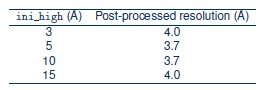
The results show that varying the initial low-pass filter has minimal effect on the final resolution. This is expected because RELION uses a gold-standard, maximum-likelihood framework in which the resolution used for alignment is determined iteratively from the data via a probability distribution, rather than being fixed by the initial reference. After the first iteration, the reference is updated from the data, and higher-resolution information is incorporated only to the extent supported by the definition of the current reconstruction. Consequently, differences in the initial low-pass filter have limited impact on the final refinement outcome.

This behavior contrasts with 2DTM, where alignment is performed by direct cross-correlation against a fixed template. In this case, high-resolution features in the template contribute directly to the scoring function and can improve alignment accuracy.

To directly test the importance of high-resolution information for 2DTM alignment, we performed an additional experiment in which 2DTM was run on bin4x images (2.234 Å/pixel), and the detected particle coordinates were used to extract particles from the corresponding bin2x images (1.117 Å/pixel) for reconstruction. Despite using the same bin2x images for reconstruction, the bin4x-aligned particles yielded a map in which ATP density was lost and backbone density for residues 222–227 was visibly degraded compared to the bin2x-aligned reconstruction (Fig. Figure 1—figure supplement 3). This demonstrates that access to high-spatial-frequency information during template matching is critical for accurate alignment of small particles.

(8) The caption in Figure 3 should be more descriptive about what is being shown in each panel.

We have substantially expanded the Figure 3 caption. It now describes each panel explicitly: (a) 3D classification results with particle counts, percentages, and per-class resolutions; (b) side-by-side comparison of reconstructions using 2DTM orientations versus RELION auto-refine, including full maps, zoomed binding-pocket views with the atomic model overlaid, orientation distributions, and FSC curves with reported resolutions; and (c) a table of RELION auto-refinement resolution as a function of the initial low-pass filter setting. We also added a new panel (c) showing that including all five classes yields the same 3.7 Å resolution, addressing the concern about Class 5 exclusion.

(9) Figures 4 and 5 may be better suited as supplementary figures.

We agree. Figures 4 and 5 have been moved to the Supplementary Information in the revised manuscript.

(10) In Figure 4c, it is difficult to understand why the thickness distribution plot goes negative, especially to such a high magnitude as 1.5 microns.

We agree this was confusing. The negative values are fitting artifacts from ctffind5’s thickness estimation, which fits a sinc-modulated envelope to the power spectrum. When the ice is very thin or the spectrum is noisy, the optimizer can converge to unphysical negative values (affecting ∼5.9% of micrographs). We have revised Figure 1—figure supplement 1c (previously Figure 4c) to show only positive thickness values, which now clearly displays the unimodal distribution peaked at 350–400 Å.

(11) In Figure 5d, the micrograph looks a lot like a cross-grating grid used for calibration instead of crystalline ice or a fractured film.

We agree. We have updated the caption for Figure 1—figure supplement 2d (originally Figure 5d) to read “Cross-grating calibration grid”

(12) Figure 6 was very surprising to me if I am interpreting it correctly. It is not stated in the caption what omega is, but I am assuming it is a measurement of template bias. It is very surprising that the template bias drops when using more particles by reducing the p-value from 8.0 to 7.0. This goes against what I understood from Lucas et al. 2023, so I am curious as to why this is the case.

We thank the reviewer for this question and apologize for the unclear presentation. We have revised Fig. 4 (previously Figure 6) and its caption to define Ω explicitly and updated the Ω values. We also identified that the mask used in the original computation was too loose; the revised mask is now constrained to the omitted region only (ATP, Mn²⁺, and residues 222–227), derived from the difference between the full and omit templates and shown in Figure 4—figure supplement 1. Ω is adapted from the template-bias metric introduced in (Lucas et al., 2023) and measures how much of the density in the omitted region is attributable to using the full template rather than the omit template. Specifically, for each particle selection condition we reconstruct two maps using orientations and particles derived from independent 2DTM searches with the full and omit templates (V_full and V_omit, respectively). Ω is the fractional reduction in density within the omission mask: . In the revised Fig. 4, Ω increases from 46% (p-value = 8.0) to 48% (p-value = 7.0), consistent with the expectation that including more, lower-quality particles increases the relative contribution of the template to the reconstruction. The Ω values are 48% for the SNR = 7.5 and 53% for the tilt conditions.

(13) It would be useful if the in-house Python script used to calculate template bias could be made publicly available.

We agree. The template-bias calculation (measure-template-bias) is now included in the publicly available Python package at https://github.com/kekexinz/2DTM_postprocess_tool, and can also be accessed in the official cisTEM repository at https://github.com/timothygrant80/cisTEM. The package also contains the extract-particles and filter-particles tools described in the Methods section.

(14) The p-value used is said to be a three-quadrant p-value instead of a one-quadrant p-value. Although I assume this is simply replacing an ‘and’ statement with an ‘or’ statement, the exact difference could be made clearer to the reader.

We have now defined these terms explicitly in the revised Methods. After probit transformation of z-score and SNR, the first-quadrant (1Q) p-value requires both values to be > 0 (logical AND), whereas the three-quadrant (3Q) p-value requires at least one to be > 0 (logical OR). The 3Q criterion is therefore looser, retaining more candidates—which is beneficial for small targets that may score well on one metric but not both.

(15) I was, perhaps naively, surprised that z-scores could not be used. It was my understanding that by removing the rotationally invariant component from the cross-correlation, the z-score would down-weight low-resolution information compared to the cross-correlation. Given that the manuscript suggests low-resolution alignment can cause getting stuck in local minima, this is surprising to me. The authors note it led to the rejection of most particles; were there simply too many false positives when a lower threshold was used?

The reviewer is correct that subtracting the angular mean removes the rotationally invariant component of the cross-correlation. However, the resulting z-score primarily measures how strongly a specific orientation stands out relative to other orientations. In other words, it reflects the orientation discriminability (closely related to Fisher information) rather than the absolute correlation strength. For small particles the cross correlation often varies only weakly across orientations, so CC_max− CC_avg remains small even when the absolute correlation is significant. As a result, using the z-score alone as a selection criterion led to the rejection of many true particles.

Theoretical Section Improvements

(a) The discussion on beam-induced motion could be improved by separating it into initial motion (e.g., cryo-crinkling, buckling) that can be eliminated through grid design, and pseudo-Brownian motion, which cannot. Pseudo-Brownian motion will become much more significant for small proteins (based on reference 5, for a 10 kDa protein, this would be a MSD of ∼0.1 A 2/e−/A 2, or a B-factor of over 2 A 2/e−/A 2), and Bayesian Polishing is unlikely to correct this perfectly, given that it imposes a smoothness of motion between nearby particles. The impact of not correcting for this could be quantified more explicitly.

We thank the reviewer for this helpful suggestion. As noted, pseudo-Brownian motion of particles within irradiated ice introduces stochastic displacements that accumulate with dose and are expected to be more significant for small particles. Based on the analysis in (Mcmullan et al., 2015), and scaling with particle size, this effect can be aproximated as a dose-dependent mean-squared displacement (MSD) of ∼0.1 Ų per (e⁻/Ų) for a ∼10 kDa particle. Over a typical total exposure of 40–60 e⁻/Ų, this corresponds to an accumulated RMS displacement of ∼2–2.5 Å, sufficient to attenuate high-resolution signal.

In practice, such motion acts as an additional high-frequency attenuation in Fourier space, analogous to an envelope function, reducing the coherent signal available for template matching. While Bayesian polishing can partially correct beam-induced motion, it assumes spatially smooth trajectories between nearby particles and therefore may not fully compensate for stochastic, particle-specific motion.

Within the theoretical framework presented here, this effect can be interpreted as an additional frequency-dependent damping of the signal (B-factor). Its primary consequence would be to reduce the effective signal-to-noise ratio at high spatial frequencies and therefore shift the detectable molecular-weight limit somewhat upward, without altering the structure of the derivation. We have added text in the manuscript to clarify this point and to indicate the expected magnitude of this effect.

(b) The inclusion of inelastic scattering assumes an energy filter is being used, and this should be clearly stated.

We have added this clarification in the inelastic scattering paragraph of the Supplementary Information.

(c) The reasons for not including other factors, such as DQE and the temporal and spatial coherence envelope functions, could be stated.

We have added a note in the dose-weighting section clarifying that these instrument-dependent attenuation factors were not explicitly included, and that they could be incorporated as additional frequency-dependent weighting terms without changing the structure of the derivation.

(d) The flexibility and heterogeneity in protein structures, especially at high spatial frequencies, must also be a reason for a gap from experiment to theory, but this is not clearly stated.

We agree. We have added a statement in the “Remaining gaps” section noting that structural flexibility and conformational heterogeneity act as an additional envelope that attenuates high-resolution signal relative to the rigid-particle model assumed in our derivation.

Additional Minor Comments

(15) It is noted in the discussion that 2DTM-based single-particle alignment simplifies the processing pipeline. Although true, I think stating the computation time would be useful for the reader.

We have added computation times to the Discussion. For a typical single-particle dataset of ∼2,000 micrographs (5k × 4k pixels), a 2DTM search without defocus refinement completes in approximately one day on 64 NVIDIA A6000 GPUs. Once particles are located with their orientations and positions, a single 3D reconstruction is sufficient without further refinement, eliminating the iterative 2D classification, ab initio modeling, 3D classification and refinement steps of a conventional pipeline.

(16) There are some formatting issues with e−/A 2, sometimes losing the minus sign.

Thank you for catching this. We have corrected all instances to consistently use e⁻/Ų throughout the manuscript.