Machine learning of dissection photographs and surface scanning for quantitative 3D neuropathology

Reviewer #1 (Public Review):

Gazula and co-workers presented in this paper a software tool for 3D structural analysis of human brains, using slabs of fixed or fresh brains. This tool will be included in Freesurfer, a well-known neuroimaging processing software. It is possible to reconstruct a 3D surface from photographs of coronal sliced brains, optionally using a surface scan as model. A high-resolution segmentation of 11 brain regions is produced, independent of the thickness of the slices, interpolating information when needed. Using this method, the researcher can use the sliced brain to segment all regions, without the need of ex vivo MRI scanning.

The software suite is freely available and includes 3 modules. The first accomplishes preprocessing steps, for correction of pixel sizes and perspective. The second module is a registration algorithm that registers a 3D surface scan obtained prior to sectioning (reference) to the multiple 2D slices. It is not mandatory to scan the surface, -a probabilistic atlas can also be used as reference- however the accuracy is lower. The third module uses machine learning to perform the segmentation of 11 brain structures in the 3D reconstructed volume. This module is robust, dealing with different illumination conditions, cameras, lens and camera settings. This algorithm ("Photo-SynthSeg") produces isotropic smooth reconstructions, even in high anisotropic datasets (when the in-plane resolution of the photograph is much higher than the thickness), interpolating the information between slices.

To verify the accuracy and reliability of the toolbox, the authors reconstructed 3 datasets, using real and synthetic data. Real data of 21 postmortem confirmed Alzheimer's disease cases from the Massachusetts Alzheimer's Disease Research Center (MADRC)and 24 cases from the AD Research at the University of Washington(who were MRI scanned prior to processing)were employed for testing. These cases represent a challenging real-world scenario. Additionally, 500 subjects of the Human Connectome project were used for testing error as a continuous function of slice thickness. The segmentations were performed with the proposed deep-learning new algorithm ("Photo-SynthSeg") and compared against MRI segmentations performed to "SAMSEG" (an MRI segmentation algorithm, computing Dice scores for the segmentations. The methods are sound and statistically showed correlations above 0.8, which is good enough to allow volumetric analysis. The main strengths of the methods are the datasets used (real-world challenging and synthetic) and the statistical treatment, which showed that the pipeline is robust and can facilitate volumetric analysis derived from brain sections and conclude which factors can influence in the accuracy of the method (such as using or not 3D scan and using constant thickness).

Although very robust and capable of handling several situations, the researcher has to keep in mind that processing has to follow some basic rules in order for this pipeline to work properly. For instance, fiducials and scales need to be included in the photograph, and the slabs should be photographed against a contrasting background. Also, only coronal slices can be used, which can be limiting for certain situations.

The authors achieved their aims, and the statistical analysis confirms that the machine learning algorithm performs segmentations comparable to the state-of-the-art of automated MRI segmentations.
Those methods will be particularly interesting to researchers who deal with post-mortem tissue analysis and do not have access to ex vivo MRI. Quantitative measurements of specific brain areas can be performed in different pathologies and even in the normal aging process. The method is highly reproducible, and cost-effective since allows the pipeline to be applied by any researcher with small pre-processing steps.

Reviewer #2 (Public Review):

Summary

The authors proposed a toolset Photo-SynthSeg to the software FreeSurfer which performs 3D reconstruction and high-resolution 3D segmentation on a stack of coronal dissection photographs of brain tissues. To prove the performance of the toolset, three experiments were conducted, including volumetric comparison of brain tissues on AD and HC groups from MADRC, quantitative evaluation of segmentation on UW-ADRC and quantitative evaluation of 3D reconstruction on HCP digitally sliced MRI data.

Strengths

To guarantee successful workflow of the toolset, the authors clearly mentioned the prerequisites of dissection photograph acquisition, such as fiducials or rulers in the photos and tissue placement of brain slices with more than one connected component. The quantitative evaluation of segmentation and reconstruction on synthetic and real data demonstrates the accuracy of the methodology. Also, the successful application of this toolset on two brain banks with different slice thicknesses, tissue processing and photograph settings demonstrates its robustness. By working with tools of the SynthSeg pipeline, Photo-SynthSeg could further support volumetric cortex parcellation. The toolset also benefits from its adaptability of different 3D references, such as surface scan, ex vivo MRI and even probabilistic atlas, suiting the needs for different brain banks.

Weaknesses

Certain weaknesses are already covered in the manuscript. Cortical tissue segmentation could be further improved. The quantitative evaluation of 3D reconstruction is quite optimistic due to random affine transformations. Manual edits of slice segmentation task are still required and take a couple of minutes per photograph. Finally, the current toolset only accepts coronal brain slices and should adapt to axial or sagittal slices in future work.

Author Response

The following is the authors’ response to the original reviews.

Reviewer 1

R1.1) Although very robust and capable of handling several situations, the researcher has to keep in mind that processing has to follow some basic rules in order for this pipeline to work properly. For instance, fiducials and scales need to be included in the photograph, and the slabs must be photographed against a contrasting background.

Our pipeline does indeed have some prerequisites in terms of data acquisition – at the very least, a ruler must be present in the photographs. A contrasting background is not strictly needed, but does definitely facilitate segmentation. We have edited the Introduction and Discussion to emphasize these prerequisites.

R1.2) Also, only coronal slices can be used, which can be limiting for certain situations.

While the 3D reconstruction based on Eq. 1 is quite general, the segmentation is indeed tailored to coronal slices of the cerebrum. As explained in the paper, this orientation is standard when slicing the cerebrum, but axial or sagittal slicing may also be of interest – particularly when dissecting the brainstem or cerebellum. We acknowledge this limitation in the Discussion of the revised manuscript.

R1.3) In the future, segmentation of the histological slices could be developed and histological structures added (such as small brainstem nuclei, for instance). Also, dealing with axial and sagittal planes can be useful to some labs.

While outside the scope of this paper, these are good ideas for future directions, and are considered in the Discussion of the revised version.

Reviewer 2

R2.1) The current method could only perform accurate segmentation on subcortical tissues. It is of more interest to accurately segment cortical tissues, whose morphometrics are more predictive of neuropathology. The authors also mentioned that they would extend the toolset to allow for cortical tissue segmentation in the future.

We agree with the reviewer that cortical parcellation has high value. We have included a new option in Photo-SynthSeg to parcellate the cortex using a machine learning block already existing in SynthSeg 2.0 (Billot et al, PNAS, 2023); see example in Figure 2 of the revised manuscript. This parcellation is volumetric; more accurate methods based on surfaces are out of the scope of this article and remain as future work. The manuscript has been edited to reflect these changes.

R2.2) Brain tissues are not rigid bodies, so dissected slices could be stretched or squeezed to some extent. Also, dissected slices that contain temporal poles may have several disjoined tissues. Therefore, each pixel in dissected photographs may go through slightly diFerent transformations. The authors constrain that all pixels in each dissected photograph go through the same aFine transform in the reconstruction step probably due to concerns of computational complexity. But ideally, dissected photographs should be transformed with some non-linear warping or locally linear transformations. Or maybe the authors could advise how to place diFerent parts of dissected slices when taking dissection photographs to reduce such non-linearity of transforms.

The reviewer is totally right. The problem with nonlinear warps is that, albeit trivial to implement, they compromise the robustness of the registration pipeline. This is because the nonlinear model introduces huge ambiguity in the space of solutions: for example, if one adds identical small nonlinear deformations to every slice, the objective function barely changes. The revised manuscript: (i) more thoroughly discussed this limitation; (ii) discusses nonlinear models for 3D reconstruction as future work; and (iii) makes recommendation about the tissue placement to minimize errors around the temporal pole.

R2.3) For the quantitative evaluation of the segmentation on UW-ARDC, the authors calculated 2D Dice scores on a single slice for each subject. Could the authors specify how this single slice is chosen for each subject? Is it randomly chosen or determined by some landmarks? It's possible that the chosen slice is between dissected slices so SAMSEG cannot segment accurately.

The slice is chosen to be close to the mid-coronal plane, while maximizing visibility of subcortical structures. The chosen slice is always a “real” dissected slice (rather than a digital “virtual” slice) and cannot be located in a gap between slices. This is clarified in the Quantitative Evaluation section of the revised manuscript.

R2.4) Also from Figure 3, it seems that SAMSEG outperforms Photo-SynthSeg on large tissues, WM/Cortex/Ventricle. Is there an explanation for this observation?

Since we use a single central coronal slice when computing Dice, SAMSEG yields very high Dice scores for large structures with strong contrast (e.g., the lateral ventricles). However, Photo-SynthSeg provides better results across the board, particularly when considering 3D analysis (see Figure 2 and results on volume correlations). We have added a comment on this issue to the revised manuscript.

R2.5) In the third experiment, quantitative evaluation of 3D reconstruction, each digital slice went through random aFine transformations and illumination fields only. However, it's better to deform digital slices using random non-linear warping due to the non-rigidity of the brain as mentioned in R2.2. So, the reconstruction errors estimated here are quite optimistic. It would be more realistic if digital slices were deformed using random nonlinear warping.

We agree with the reviewer and, as we acknowledge in the manuscript, the validation of the reconstruction error with synthetic data is indeed optimistic. The problem with adding nonlinear warps is that the results will depend heavily on the strength of the simulated deformation. We keep the warps linear as we believe that the value of this experiment lies in the trends that the errors reflect, as a function of slice thickness and its variability (“jitter”). This has been clarified in the revised manuscript.

Reviewer 2 (recommendations for the authors)

AR2.1) In the abstract, the authors mentioned that the segmentations of the 3D reconstructed stack deal with 11 brain regions, however, in most sections, only 9 tissue masks were compared, such as in Table 1, 2, and Figure 3. Also in the supplementary video, there are only 10 rendered tissues. So, what are these 11 regions? Is the background nonbrain region also counted as a region? And how these 11 regions were derived from the original 36 annotated tissues in T1-39?

We particularly thank the reviewer for noticing this.

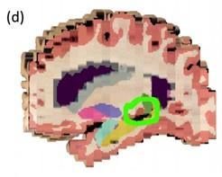
The 11 regions are white matter, cortex, ventricle, thalamus, caudate, putamen, pallidum, hippocampus, amygdala, accumbens area, and ventral diencephalon. These are all bilateral labels, i.e., 22 regions in total. The original 36 labels include these 22 and: four labels for the cerebellum (left and right cortex and white matter); the brainstem; five labels for cerebrospinal fluid regions that we do not consider; the left and right choroid plexus; and two labels for white matter hypo intensities in the left and right hemisphere.

As in many other papers, we leave “ventral diencephalon” and “accumbens area” out of the validation as they are not very well defined.

We note that all regions except the accumbens are visible in Figure 1d. The ventral diencephalon is easy to miss as only a small portion of it is visible (when picking a slice, one needs to compromise in terms of how much of each structure is visible). Moreover, it has a very similar color to the cortex in the FreeSurfer convention (see picture below).

Author response image 1.

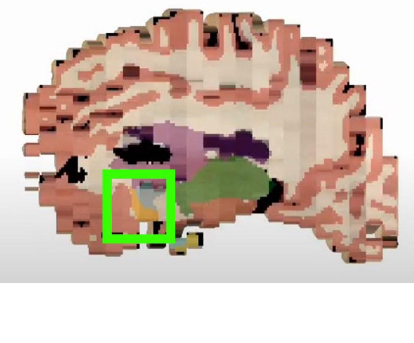
The accumbens is visible at 1m45s in the, segmented in orange (see capture below).

Author response image 2.

We have clarified these issues in the reviewed version of the manuscript.

RA2.2) In Figure 1(f), why are the hippocampal volumes of confirmed AD subjects larger than those of the healthy controls? Is this a typo or is there any explanation for this?

Yes, it is a typo. Again, thank you very much for noticing this.

RA2.3) Typo on P3, "sex and gender were corrected" should be "age and gender were corrected".

This has been corrected in the revised version.

RA2.4) In the MADRC dataset, the authors mentioned that there are 18 full brains and 58 hemispheres, however, the total data size is 78. Is this a typo?

Yes, it is. It has been corrected in the revised version.

RA2.5) Comparing the binary masks in Figure 5(d) and the photographs in Figure 5(c), some tissues below the ventricles with high intensities are also removed from masks. Is this done by manual editing? If so, how long does it usually take to edit a clean mask for each subject?

We used a combination of thresholding, morphological operations (erosion/dilation), and minor manual edits when needed – particularly to remove chunks of pial surface when they are visible, in the most anterior slices. The average is a couple of minutes per photograph. In the future, we plan to use these manually curated images to train a supervised convolutional neural network to perform the task automatically. These details are provided in the revised manuscript.

RA2.6) In the method of 3d reconstruction, there are four weights for the optimization function. How did the authors determine such weights and do these weights have some impact on the reconstruction performance?

The parameters were set by visual inspection of the output on a small pilot dataset, and do not have a strong impact on the reconstruction. The crucial aspect is to increase 𝜈 (the affine regularizer) and decrease 𝛼 (compliance with the external reference) when using a soft reference. These details have been added to the revised version.

RA2.7) Finally for the deep learning-based segmentation, a U-Net was trained on GMM generated single-channel intensity synthetic images while the dissected photographs are color images with three channels. So, did the authors only input the grayscale photographs to the segmentation network? Are there any other preprocessing steps for color photographs, such as normalization? Is it possible to use GMM to generate color images as training data to better suit dissection photography?

We did try simulating three channels during training, but the performance was actually worse than when simulating one channel and converting the RGB input to grayscale. This information has been added to the revised version.