Changing the responses of cortical neurons from sub- to suprathreshold using single spikes in vivo
- Max Planck Institute for Biological Cybernetics, Germany
- Brain Mind Institute, Ecole Polytechnique Federale de Lausanne, Switzerland
- Bernstein Center for Computational Neuroscience, Germany
Figures
Figure 1
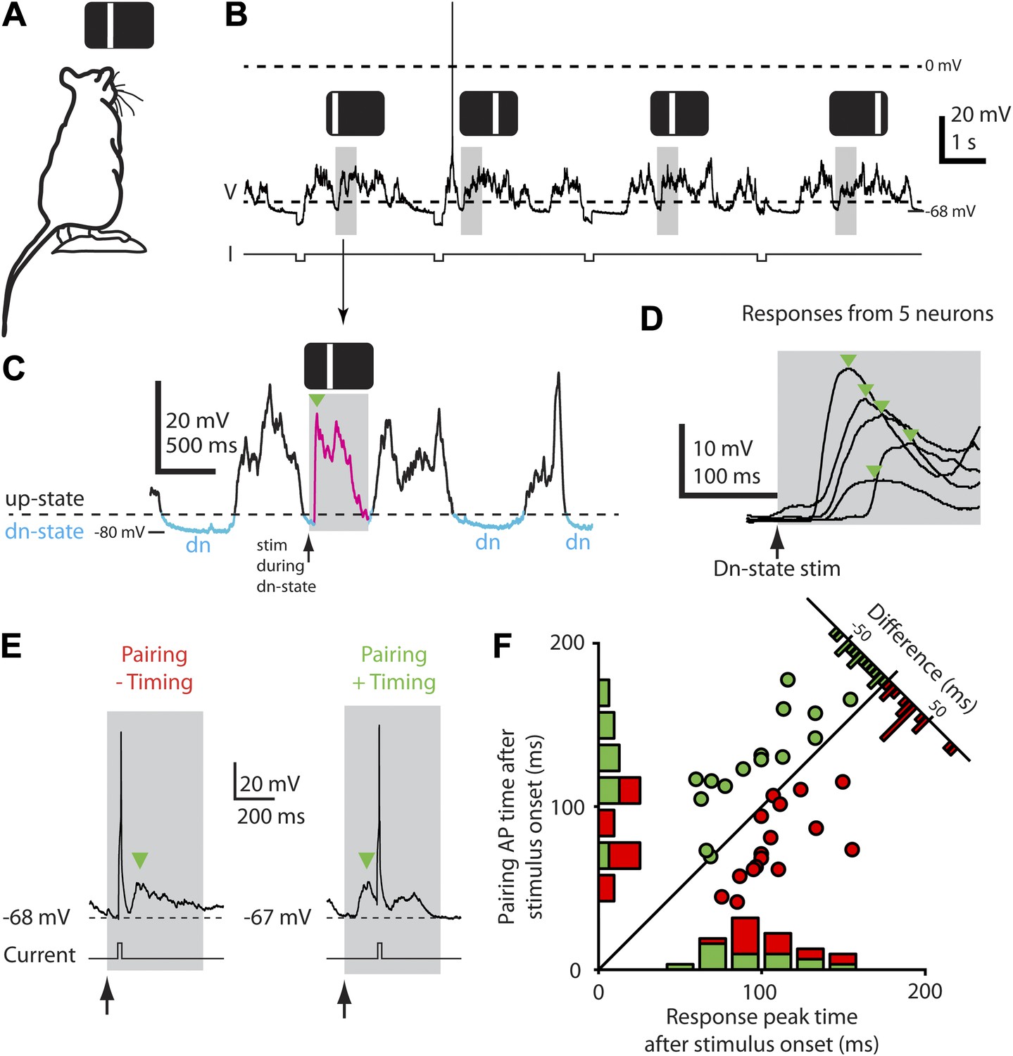
Down-state triggering of visual stimuli and timing of evoked responses and spikes during the STDP protocol.
(A) Flashed vertical bars were presented to an anesthetized rat from a stimulus screen. (B) Continuous whole-cell current-clamp recording with down-state triggered visual stimulus presentations (grey boxes) and hyperpolarizing step currents (−100 pA) to estimate input resistance. Flashed vertical bars were presented in one of four different positions across the stimulus screen. (C) Detailed view of whole-cell current-clamp recording of a voltage response (magenta, green arrow marks initial peak) to a 500 ms (grey box) flashed bar presented only during down-states (period marked in blue, dashed line indicates threshold used for online down-state detection). (D) Average membrane potential responses (green arrows indicate initial response peaks) to flashed bar stimulus for five different neurons. (E) Pairing consisted of injecting depolarizing current into the postsynaptic neuron to elicit a single AP timed to occur either before (left, ‘−Timing’) or after (right, ‘+Timing’) the response peak (green arrow). (F) Scatter plot showing timing of evoked APs for each recording vs timing of initial response peak (n = 32). Time 0 denotes stimulus onset. Histograms show the number of neurons with positive timing and negative timing.
Figure 2
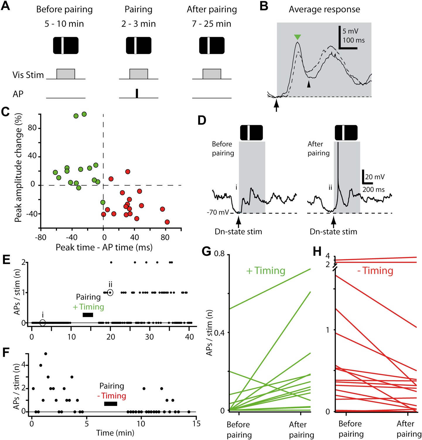
STDP converts subthreshold responses to visual stimuli into suprathreshold responses.
(A) Time course of the experiment. Before the pairing, responses to visual stimulation were recorded, during the pairing, visual stimulation was paired with APs evoked by brief current injection (repeated 40 times), followed by recording of visual responses. (B) Average membrane potential responses to stimulus presentation at the pairing position, before (dashed line) and after pairing (black line). The portion of the response before the pairing APs are potentiated, while the portion after is depressed. Small black arrow indicates timing of pairing APs. (C) Scatter plot showing the change in peak amplitude vs the time difference between the pairing APs relative to the peak. Delivering APs before the peak (red circles) decreases the peak amplitude, while delivering them after increases it (green circles). (D) Subthreshold membrane potential response to flashed bar (grey box) before pairing with a postsynaptic spike after the initial peak (positive timing), and suprathreshold response to same flashed bar stimulus after pairing. (E) Number of APs evoked per visual stimulus before and after pairing, for the neuron shown in (D). (F) Number of APs evoked per visual stimulus before and after pairing, for a neuron that received a negative timing protocol (postsynaptic spike before the initial peak). (G) Average number of APs evoked per stimulus before pairing compared to after pairing for all neurons with positive timing induction (n = 15). (H) Average number of APs evoked per stimulus before pairing compared to after pairing for all neurons with negative timing induction (n = 17).
Figure 3

Changes in sensory-evoked spiking are stimulus-specific and lead to spatial reorganization of neurons' stimulus responses.
(A) Stimulus-AP pairing was performed for a single stimulus position, but responses to neighboring and more distant positions were also measured before and after the pairing phase of the experiment. (B) Number of APs evoked per visual stimulus before and after pairing with positive timing. Stimulus-evoked spiking is shown for the paired position (upper), a neighboring position (center) and a more distant position (lower). The increase in stimulus-evoked spiking is greatest at the paired position, and the size of the change decays with distance. (C) As in (B), but showing an example where the paired position displays an increase in firing (upper) while a more distant position displays a decrease (lower). (D) Rates of spiking evoked by sensory stimulation in the recording shown in (B), before and after pairing (paired position marked by grey box); vertical arrows indicate direction of the change from before to after pairing. Dashed vertical lines indicate the suprathreshold stimulus response center before and after pairing, which shifted from position 1.00 to 2.86. (E) As in (D), but for the recording shown in (C), where a more distant position decreased its rate of stimulus-evoked spiking; response center shifted from 3.62 to 2.06. (F) Shifts in the suprathreshold stimulus response center after the pairing. Each arrow indicates the response center positions before and after pairing for a single experiment with positive (green) or negative timing (red). Vertical positions of arrows are arbitrary. Note that suprathreshold response center shifts could not be calculated for some recordings with insufficient spiking (see ‘Materials and methods’). Positive timing experiments display a shift toward the paired position. (G) Increase in stimulus-evoked spiking for neurons receiving positive timing inductions, as a function of distance from the paired position. Asterisks indicate significance at the p<0.05 level (Wilcoxon rank sum test).
Figure 4
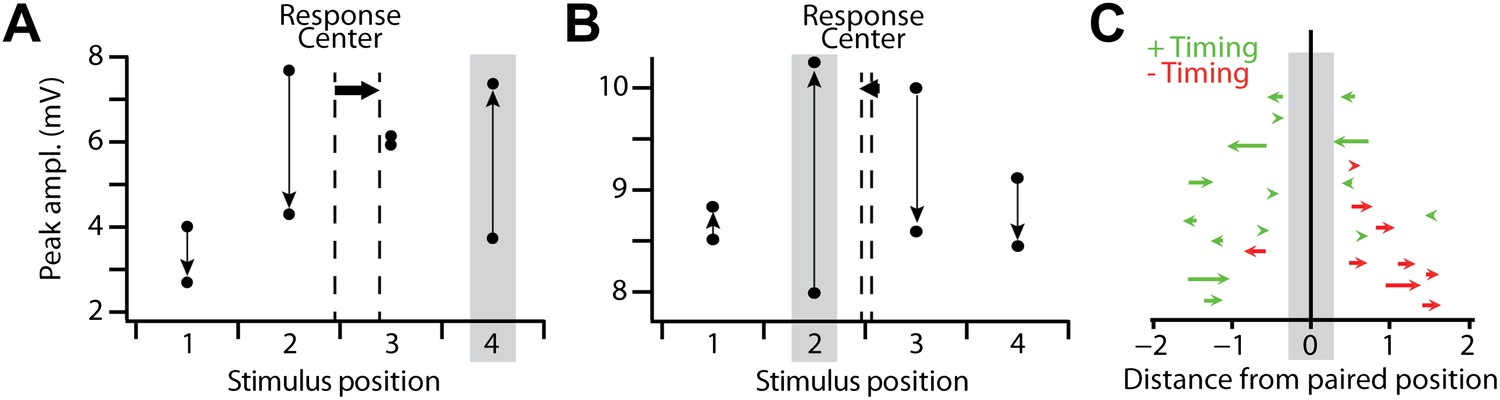
Spatial reorganization of subthreshold responses.
(A) Mean amplitude of the subthreshold response peak in a single recording with a positive timing induction, for all stimulus positions before and after pairing. Grey box indicates the pairing position, vertical arrows indicate the direction of the change from before to after pairing, and dashed vertical lines the subthreshold stimulus response center before and after pairing, which shifted from position 2.44 to 2.89 (horizontal arrow). (B) As in (A), but for a recording in which subthreshold responses at the pairing position transitioned from weakest of the four positions to strongest after pairing; response center shifted from 2.55 to 2.46. (C) Shifts in the subthreshold stimulus response center after stimulus-AP pairing, for positive timing inductions (green) and negative timing inductions (red). Each arrow indicates the response center positions before and after pairing for a single experiment with positive (green) or negative timing (red). Vertical positions of arrows are arbitrary.
Figure 5 with 3 supplements
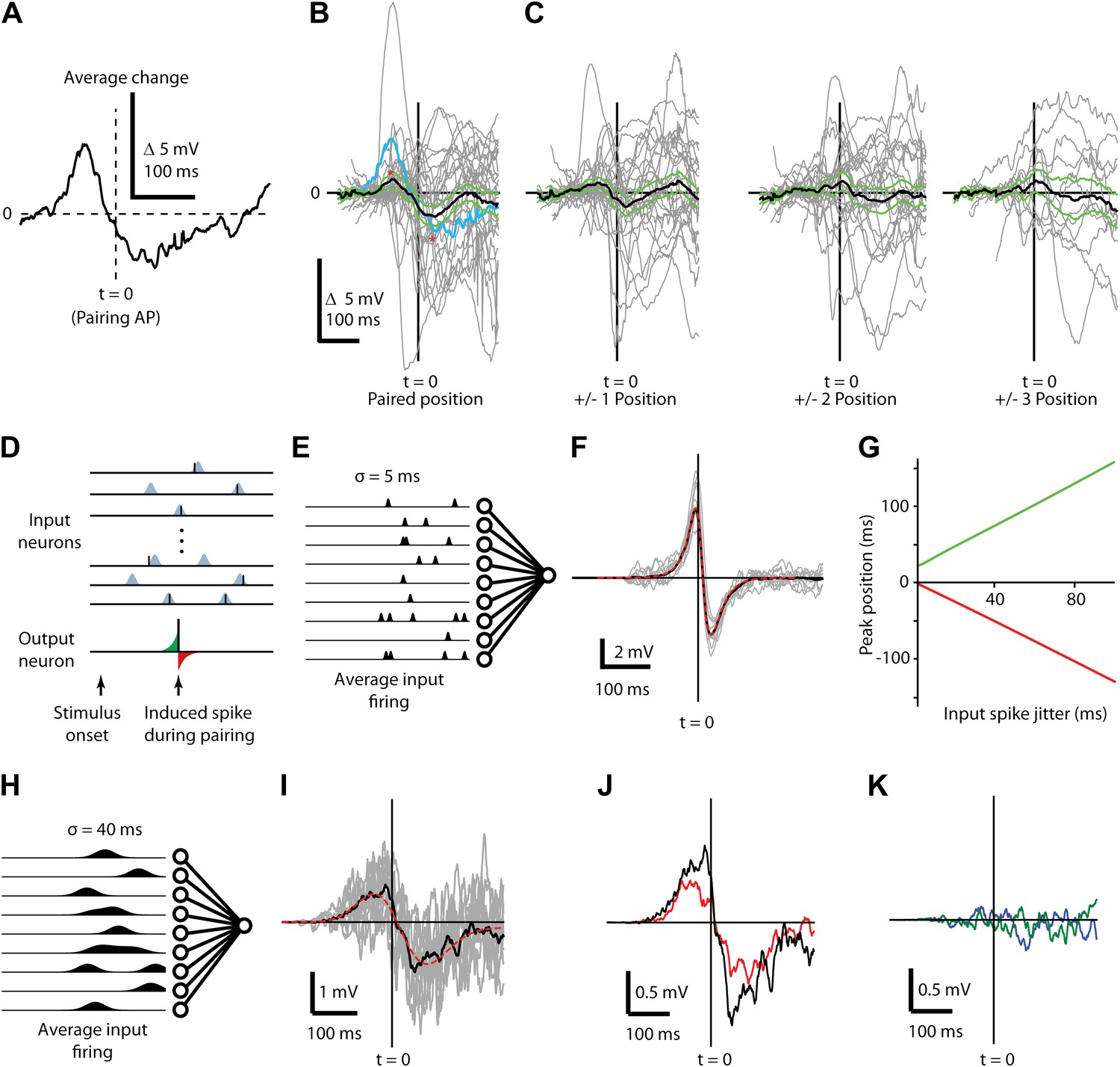
Changes in subthreshold responses after STDP induction display temporally broad peaks consistent with pre-synaptic jitter.
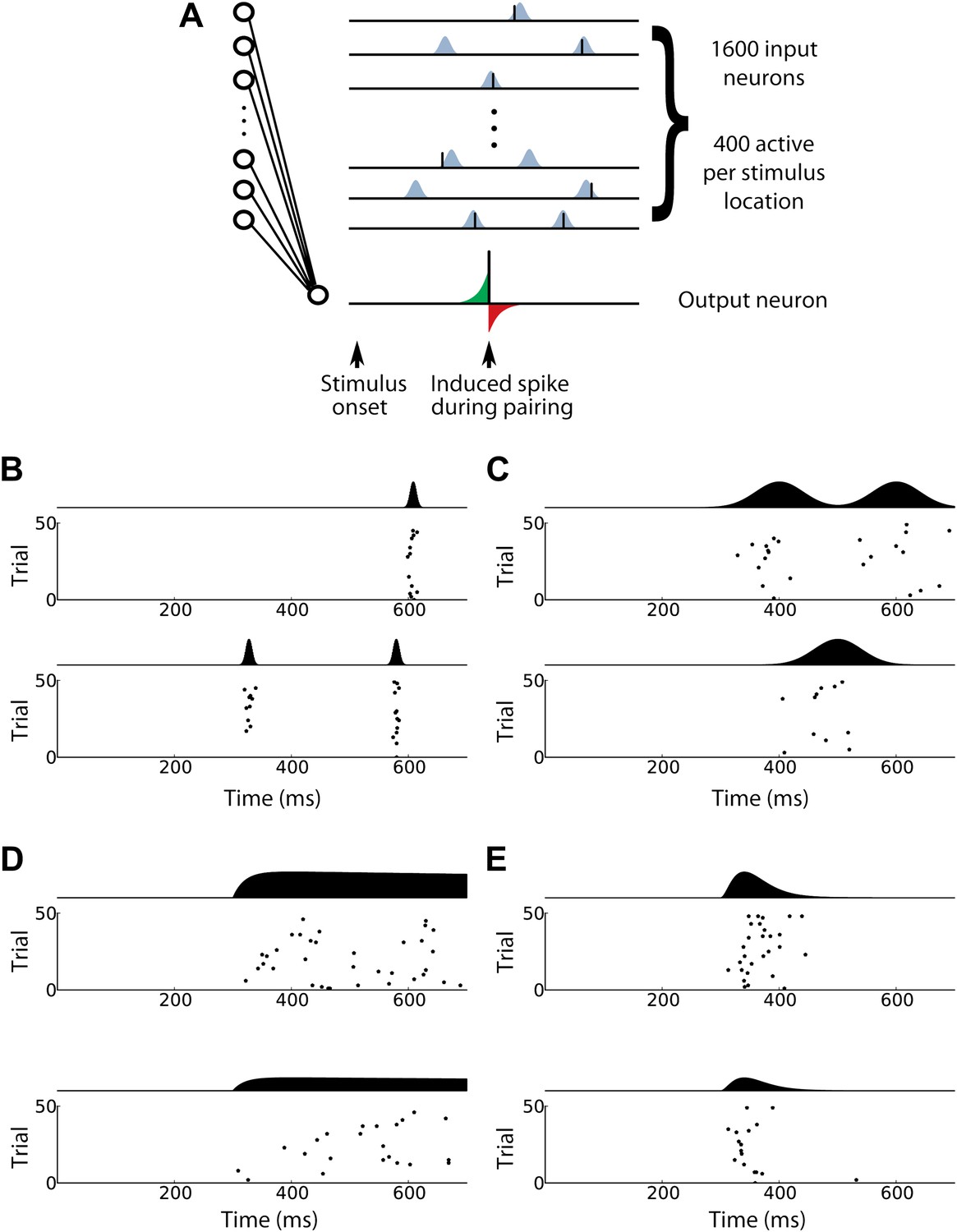
(A) Average difference between before and after pairing membrane potential time course in response to visual stimulation at the paired position for a single neuron, aligned to the time of the pairing spike (dashed vertical line, t = 0). (B) Average (black) difference between before and after pairing membrane potential response to visual stimulation, as a function of time difference from the pairing spike. Individual neurons are shown in grey, green lines indicate SEM and the example neuron from (A) is shown in blue. (C) As in (B), but for non-paired stimulus positions adjacent to the paired position (left) and more distant positions (center, right). (D) Structure of the computational model showing that for each stimulus 400 presynaptic neurons were activated, providing input to a single postsynaptic neuron. Input spikes had a Gaussian probability distribution around target firing times. During pairing, a single postsynaptic spike (bottom) is induced at a predetermined time and input weights are increased if an input spike arrives at the respective synapse just before the induced spike (green area) and decreased if an input spike occurs just after the induced spike (red area). (E) Schematic showing mean firing rates over time for input neurons with σ = 5 ms used for calculating F. (F) Average difference in membrane potential when the input spike precision is ∼5 ms (individual simulations grey, mean red) compared to a theoretical curve. (G) Timing of the positive (green) and negative (red) peaks of the membrane potential change relative to the induced postsynaptic spike as a function of the jitter in input spike timing. (H) Schematic showing mean firing rates over time for input neurons with σ = 40 ms used for calculating I. (I) Average difference in membrane potential when the input spike precision is ∼40 ms. (J) Transfer of plasticity to a neighboring stimulus position when a subpopulation of synapses and timing are shared (red) compared to membrane potential difference from (I, black). (K) Transfer of plasticity to a neighboring stimulus position when a subpopulation of synapses are shared but timing is not (blue), and when no synapses are shared (green).
Figure 5—figure supplement 1
Input spike patterns for the computational model of in vivo STDP effects.
(A) (Left) Structure of the computational model. For each stimulus, 400 presynaptic input neurons are activated and each sends zero, one, or several spikes to a single postsynaptic output neuron. (Upper right) Schematic diagram illustrating input spike trains using patterned spike timing (see ‘Input spike patterns’ in ‘Materials and methods’). Spike times are Gaussian-distributed around target times from a fixed template that is different for each input neuron. During pairing, a single postsynaptic spike (lower right) is induced at a fixed time. Synapse strengths are updated according to a STDP rule, increasing when an input spike arrives at the respective synapse briefly before the induced spike (green area) and decreasing when an input spike occurs briefly after the induced spike (red area). (B)–(E) Various activity patterns used to model the firing of presynaptic input neurons. Each panel shows raster plots and mean firing rates over time for two input neurons. (B) Inputs with patterned spike timing and 5 ms jitter produce precisely timed activity patterns. (C) Patterned spike timing with 40 ms jitter is less temporally precise. (D) The time varying firing rates scheme exhibits a clear onset time and a different maximum firing rate for each neuron. (E) The activity wave scheme exhibits rapid decay in firing rates after the maximum rate has been reached.
Figure 5—figure supplement 2
Membrane potential responses in the postsynaptic output neuron for various activity patterns used to model the firing of presynaptic input neurons.
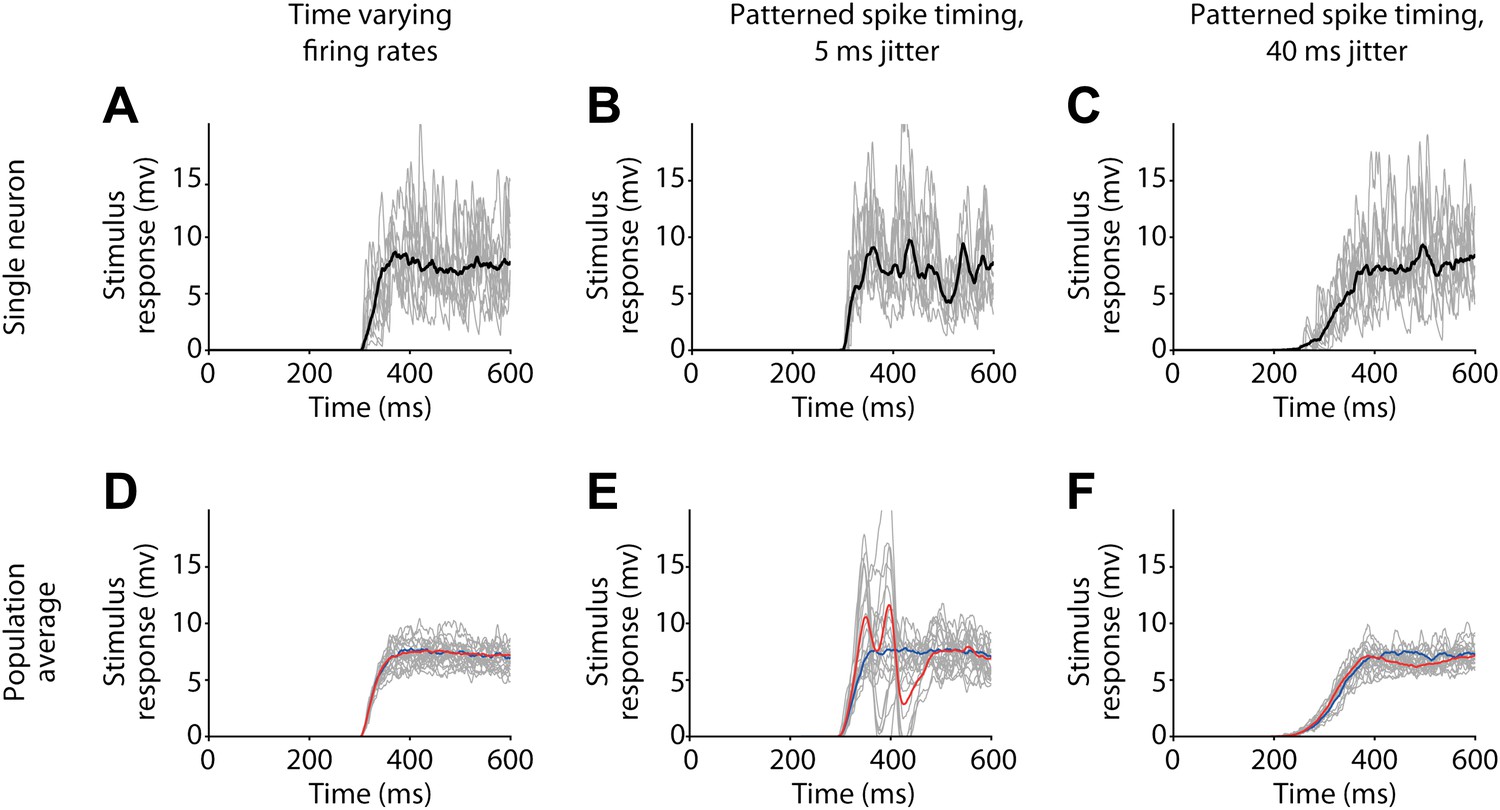
(A)–(C) Responses of a single postsynaptic neuron to individual stimulus presentations (grey) and average response (black), before pairing. (A) Time varying firing rates. (B) Patterned spike timing with 5 ms jitter. (C) Patterned spike timing with 40 ms jitter. (D)–(F) Mean responses from all simulated postsynaptic neurons (grey) and combined population averages before (blue) and after pairing (red) (population averages computed over 9 neurons with negative timing simulations 15 with positive timing simulations). (D) Time varying firing rates. (E) Patterned spike timing with 5 ms jitter. (F) Patterned spike timing with 40 ms jitter.
Figure 5—figure supplement 3
Changes in membrane potential responses to stimulus presentation after pairing for all activity patterns used to model the firing of presynaptic input neurons.
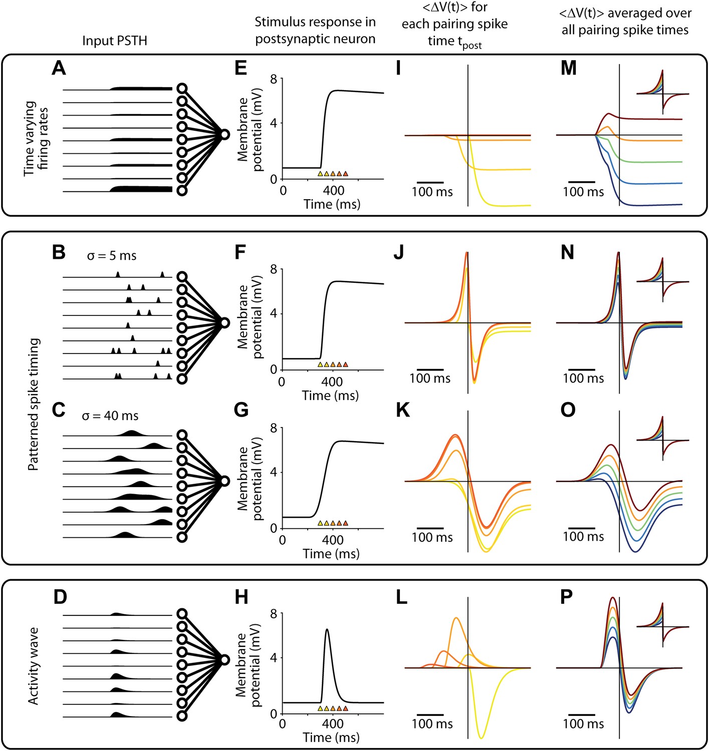
(A)–(D) Mean firing rates over time for input neurons (see Figure 5—figure supplement 1 for details). (E)–(H) Input spikes converge on the output neuron and elicit a membrane potential response, (schematic shown, see Figure 5—figure supplement 2 for simulation results). Colored triangles indicate potential timings of postsynaptic spikes in simulated pairing experiments. (I)–(L) Time course of changes in the membrane potential response relative to the time of the pairing spike (t = 0). Results depends on the time of the pairing spike (colors correspond to triangles in (E–H), with yellow around response onset and red after response peak). (M)–(P) Time course of changes in the membrane potential response relative to the time of the pairing spike (t = 0), averaged over two different timings for the pairing spike (see ‘Simulation protocol’ in ‘Materials and methods’). Results are shown for various values of A(−) in the STDP learning window (see inset; A(+) = 0.2, A(−) = 0.16, 0.18, 0.2, 0.22 or 0.24).
Download links
A two-part list of links to download the article, or parts of the article, in various formats.
Downloads (link to download the article as PDF)
Open citations (links to open the citations from this article in various online reference manager services)
Cite this article (links to download the citations from this article in formats compatible with various reference manager tools)
Changing the responses of cortical neurons from sub- to suprathreshold using single spikes in vivo
eLife 2:e00012.
https://doi.org/10.7554/eLife.00012


