Diagnostically relevant facial gestalt information from ordinary photos
- University of Oxford, United Kingdom
- The Wellcome Trust Centre for Human Genetics, University of Oxford, United Kingdom
- Institute of Genetics and Molecular Medicine, United Kingdom
Figures
Figure 1 with 2 supplements
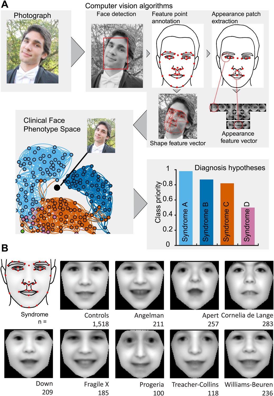
Overview of the computational approach and average faces of syndromes.
(A) A photo is automatically analyzed to detect faces and feature points are placed using computer vision algorithms. Facial feature annotation points delineate the supra-orbital ridge (8 points), the eyes (mid points of the eyelids and eye canthi, 8 points), nose (nasion, tip, ala, subnasale and outer nares, 7 points), mouth (vermilion border lateral and vertical midpoints, 6 points) and the jaw (zygoma mandibular border, gonion, mental protrubance and chin midpoint, 7 points). Shape and Appearance feature vectors are then extracted based on feature points and these determine the photo's location in Clinical Face Phenotype Space (further details on feature points in Figure 1—figure supplement 1). This location is then analyzed in the context of existing points in Clinical Face Phenotype Space to extract phenotype similarities and diagnosis hypotheses (further details on Clinical Face Phenotype Space with simulation examples in Figure 1—figure supplement 2). (B) Average faces of syndromes in the database constructed using AAM models (‘Materials and methods’) and number of individuals which each average face represents. See online version of this manuscript for animated morphing images that show facial features differing between controls and syndromes (Figure 2).
Figure 1—figure supplement 1
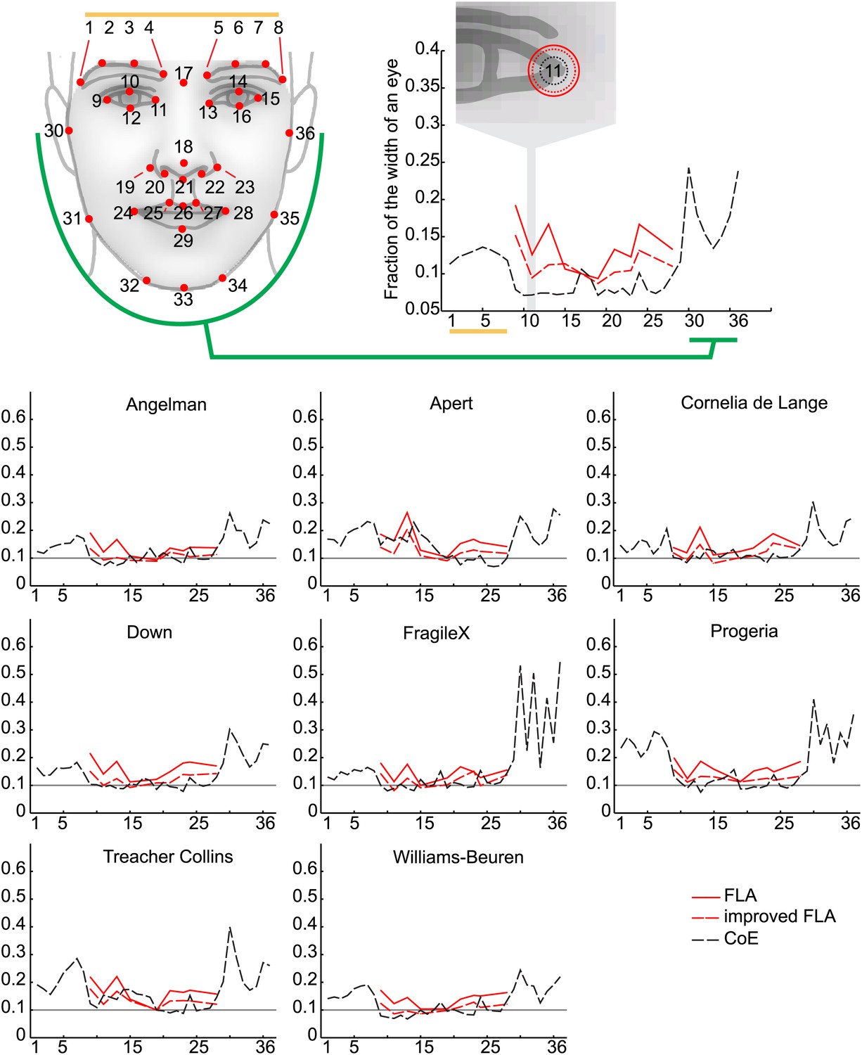
(A) The 36 facial feature points annotated by the automatic image analysis algorithm. Supra-orbital ridge (8 points), the eyes (mid points of the eyelids and eye canthi, 8 points), nose (nasion, tip, ala, subnasale and outer nares, 7 points), mouth (vermilion border lateral and vertical midpoints, 6 points), and the jaw (zygoma mandibular border, gonion, mental protrubance and chin midpoint, 7 points). (B) The annotation accuracies relative to the manually annotated ground truth of each of the computer vision modules. Points 1–8 refer to the supra-orbital ridge, points 30–36 refer to the jaw points. Accuracies for the points annotated by the modules FLA, improved FLA and CoE are shown for each syndrome and control groups. Accuracies are shown as the average error relative to the width of an eye.
Figure 1—figure supplement 2
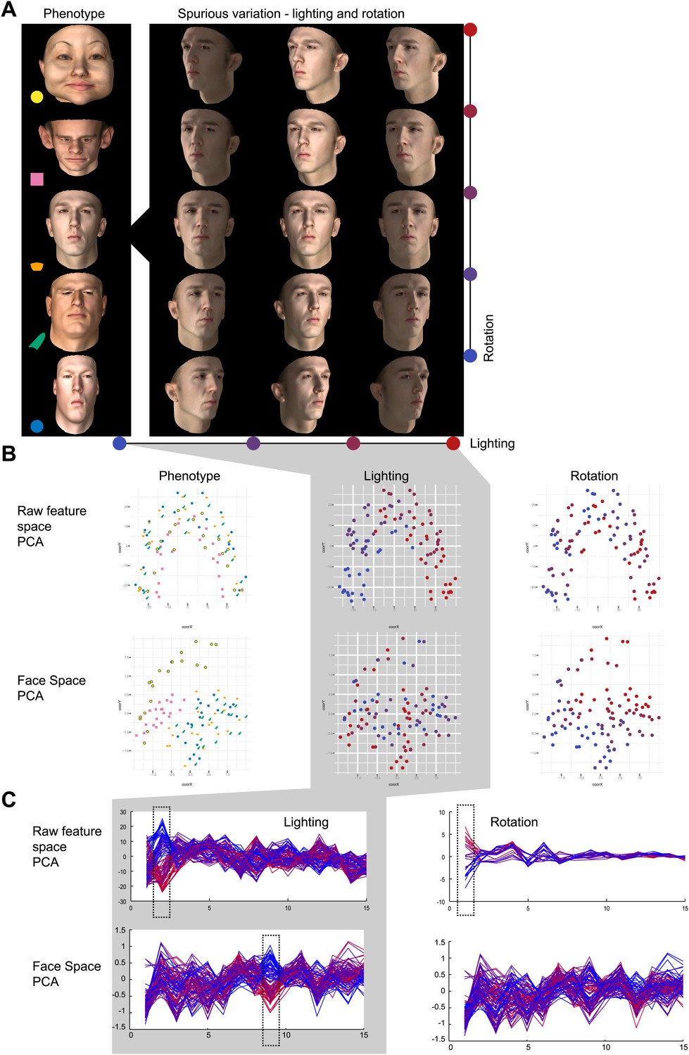
Phenotypic vs spurious feature variation in Clinical Face Phenotype Space using simulated faces.
Simulated 3D faces were used to visualize the influence of spurious variation in raw feature space and Clinical Face Phenotype Space. (A) 100 faces with controlled phenotype, lighting, and rotation variation were rendered. (B) Visualization of a population of simulated faces in the first two Multi-Dimensional Scaling (MDS) modes. Face clustering in raw feature space and Clinical Face Phenotype Space colored by lighting, rotation, and face phenotype, respectively. In the raw feature space lighting is the dominating clustering factor, in Clinical Face Phenotype Space phenotype underlies the primary clustering. (C) The first 16 modes of PCA decomposition of the raw feature vectors and in the Clinical Face Phenotype Space colored by lighting and rotation of the simulated faces. In the raw feature space, lighting, and rotation variation are encoded in the 2nd and 1st modes, indicating that clustering is dominated by spurious variation. In the Clinical Face Phenotype Space, lighting is represented in the 9th mode, whereas rotation is no longer represented in the first 16 modes. This shows that the Clinical Face Phenotype Space transformation reduces the influence of spurious variation on clustering of phenotypes.
Figure 2—figure supplement 1
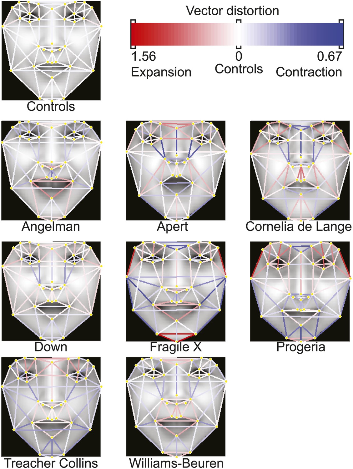
Distortion graphs representing the characteristic deformation of syndrome faces relative to the average control face.
Each line reflects whether the distance is extended or contracted compared with the control face. White—the distance is similar to controls, blue—shorter relative to controls, and red—extended in patients relative to controls.
Figure 3
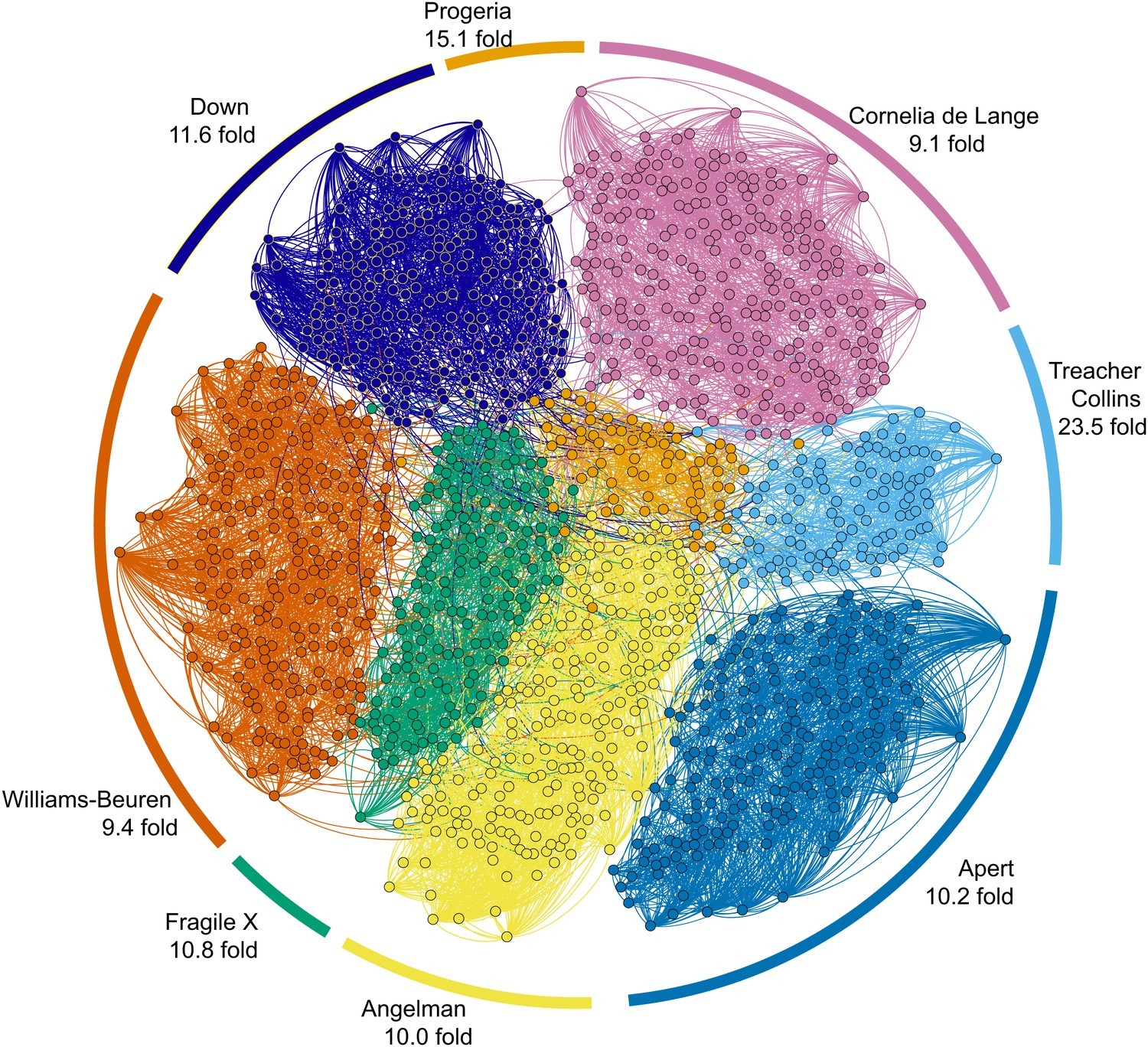
Clinical Face Phenotype Space enhances the separation of different dysmorphic syndromes.
The graph shows a two dimensional representation of the full Clinical Face Phenotype Space, with links to the 10 nearest neighbors of each photo (circle) and photos placed with force-directed graphing. The Clustering Improvement Factor (CIF, fold better clustering than random expectation) estimate for each of the syndromes is shown along the periphery.
Figure 4 with 4 supplements
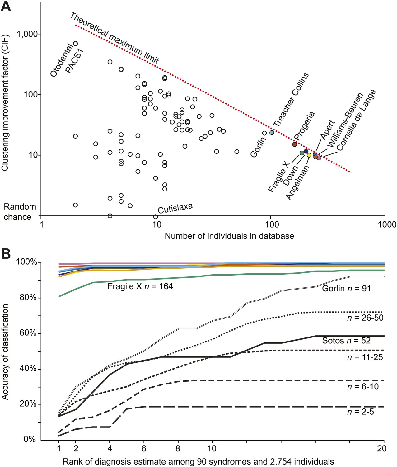
Clinical Face Phenotype Space is generalizable to dysmorphic syndromes that are absent from a training set.
(A) Clustering Improvement Factor (CIF) estimates are plotted vs the number of individuals per syndrome grouping in the Gorlin collection or patients with similar genetic variant diagnoses. As expected, the stochastic variance in CIF is inversely proportional to the number of individuals available for sampling. The median CIF across all groups is 27.6-fold over what is expected by clustering syndromes randomly. That is to say, the CIF of a randomly placed set is 1. The maximum CIF is fixed by the total number of images in the database and by the cardinality of a syndrome set: the theoretical maximal CIF upper bound is plotted as a red dotted line. The CIF for the minimum and maximum, Cutislaxa syndrome and Otodental syndrome, were 1.0 and 700.0 respectively. (B) Average probabilistic classification accuracies of each individual face placed in Clinical Face Phenotype Space (class prioritization by 20 nearest neighbors weighted by prevalence in the database). The 8 initial syndromes used to train Clinical Face Phenotype Space are shown in color. For syndromes with fewer than 50 examples, accuracies were averaged across all syndromes binned by data set size (i.e., the average accuracy is shown for syndromes with 2–5, 6–10, 11–25, and 26–50 images in the database, Supplementary file 1). Classification accuracies increase proportional to the number of individuals with the syndrome present in the database. Accuracies using support vector machines with binary and forced choice classifications are shown in Figure 4—figure supplement 1 and Figure 4—figure supplement 2. A simulation example of probabilistic querying of Clinical Face Phenotype Space is shown in Figure 4—figure supplement 3.
Figure 4—figure supplement 1

SVM binary classification accuracies among the 8 syndromes in Table 1.
SVM classifier accuracies when tuned for equal false positive and false negative error rates.
Figure 4—figure supplement 2

SVM forced choice classification accuracies among the 8 syndromes in Table 1.
https://doi.org/10.7554/eLife.02020.013
Figure 4—figure supplement 3
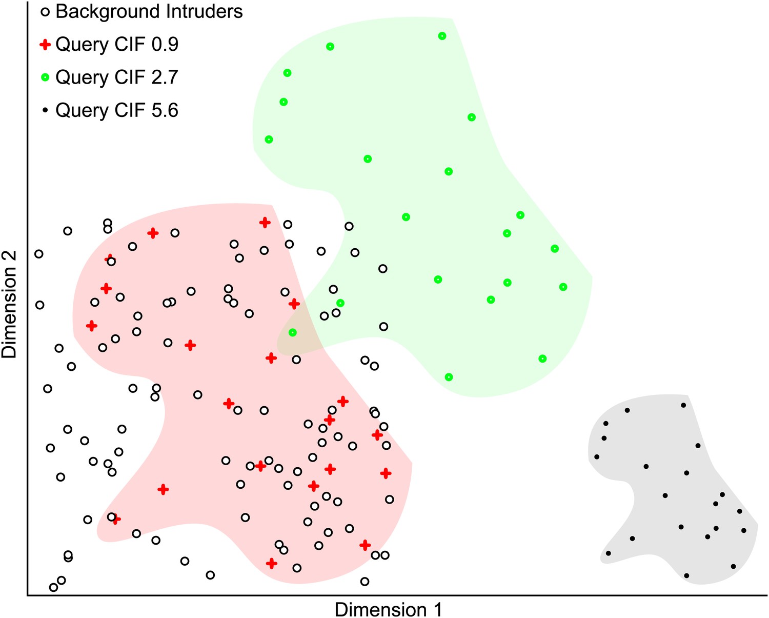
Simulated example illustrating the Clustering Improvement Factor.
A random scattering of 100 points in 2 dimensions is used as a background set (black circles with white fill). The 20 red plus symbols (within the red shaded area) are a random set of points lying within the same limits as the background set and have a CIF of 0.9. This is the actual degree of clustering of the red points with respect to the expectation of clustering them with 95% confidence (E(r) = 5.6). The filled green circles (within the green shaded area) are the red points shifted by +0.5 units in each dimension and have a CIF of 2.7. The black points (within the gray shaded area) are the red plus symbol positions scaled by 0.5 and then shifted by +1.5 units in dimension 1. The black points are non-overlapping with the background and represent the maximal CIF (of 5.6) in this example.
Figure 4—figure supplement 4
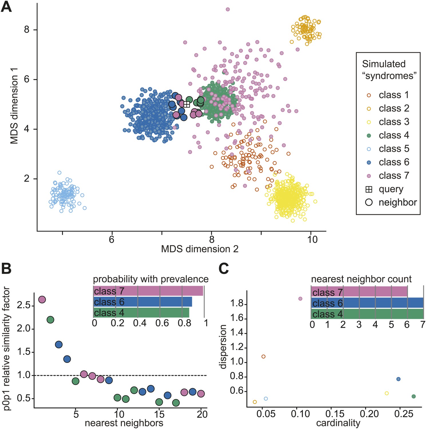
Simulated example of probabilistic querying of Clinical Face Phenotype Space.
(A) Visualization of a population of simulated faces in the first two Multi-Dimensional Scaling (MDS) modes. 7 classes of points (simulated 'syndrome groups') are shown with different distributions and variances. A central 'query' face is indicated by the boxed cross. The 20 nearest neighbors of the query are encircled with a black border. (B) Inset bar graph shows diagnosis hypothesis ranked by class priority. The class priority ranking weights the dispersion and prevalence (spread and number) of a class in the Clinical Face Phenotype Space with the nearest neighbors to assign the most probable diagnosis hypotheses. In the example, the ranked diagnosis estimates of the query point would be class 7, then class 6, and thirdly class 4. The scatter plot shows the individual similarity p0p1 estimates, reflecting their relative closeness in the space as compared to local neighborhood, for the 20 nearest neighbors of the query. The first nearest neighbor is estimated to be 2.6-fold closer to the query than the average based on the local density of neighbors. The dotted line indicates the average relative distance between points among the 20 nearest neighbors. (C) Inset bar graph shows the number of neighbors of the query per class. A scatterplot of dispersion vs cardinality, i.e. relative spread of points and what proportion of the total number of points belong to that class in the simulated space. Plots (B) and (C) allow objective assessment of the distribution of points shown in (A), and aid the interpretation of classification confidence.
Figure 5
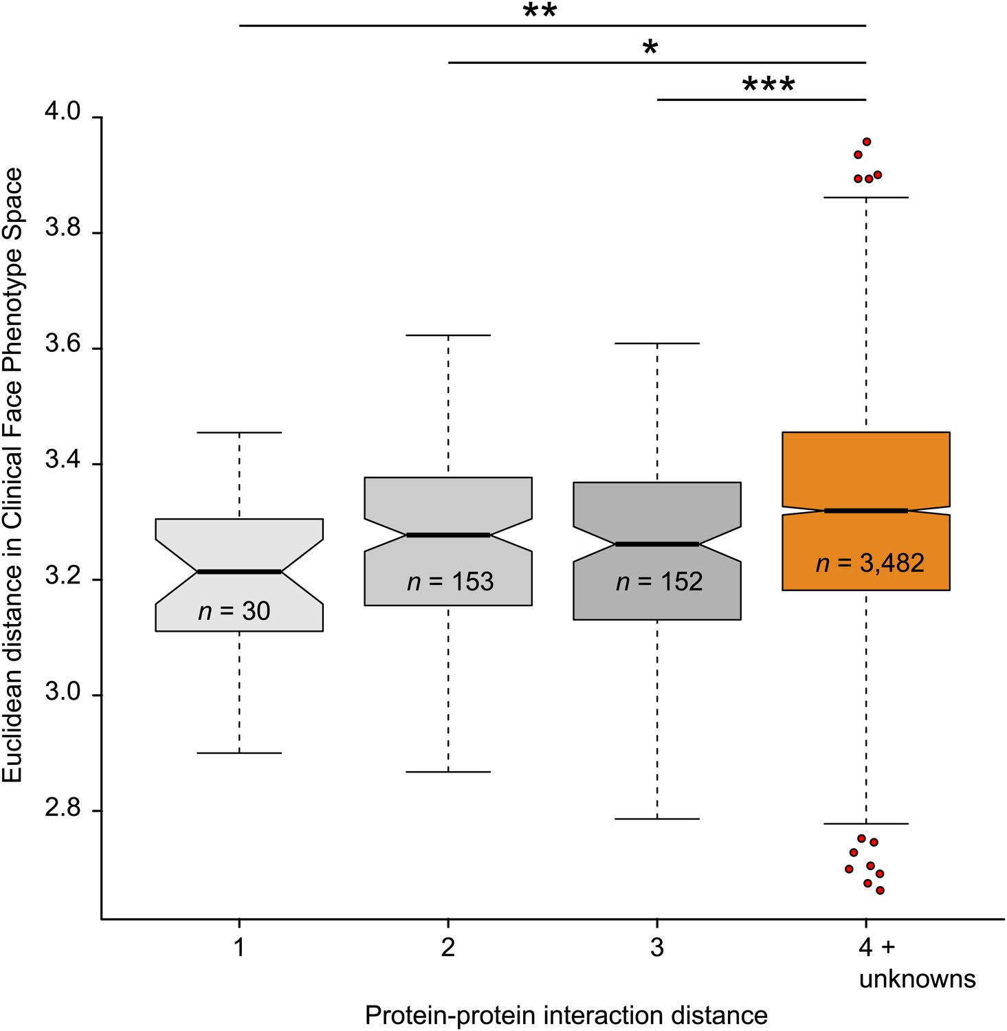
Clinical Face Phenotype Space recapitulates features of functional gene links between syndromes.
Protein–protein interaction distances of 1–3 for genetically characterized syndromes are associated with significantly shorter Euclidean distance (arbitrary units) between syndromes in Clinical Face Phenotype Space as compared to syndromes with distance 4 or no known interaction distance (shown in orange) (Kruskal–Wallis tests with Bonferroni corrected p-values indicated as *p<0.05, **p<0.01, ***p<0.001). The Spearman correlation across all distances was r = 0.09, p<0.001. The numbers of pairwise syndrome comparisons underlying each of the interaction distances are listed within the respective boxes.
Figure 6

Class priority of diagnostic classifications for images.
The full computer vision algorithm and Clinical Face Phenotype Space analysis procedure with diagnostic hypothesis generation exemplified by: (A) a patient (Ferrero et al., 2007) with Williams-Beuren. (B) Abraham Lincoln. The former US President is thought to have had a marfanoid disorder, if not Marfan syndrome (Gordon, 1962; Sotos, 2012). Bar graphs show class prioritization of diagnostic hypotheses determined by 20 nearest neighbors weighted by prevalence in the database. As expected, the classification of Marfan is not successfully assigned in the first instance as there were only 18 faces of individuals with Marfan in the database (making this an example of a difficult case with the current database). However, the seventh suggestion is Marfan, despite this being among 90 different syndromes and 2754 faces.
© 2007 Elsevier Masson SAS. All rights reserved. The patient figure in Figure 6, part A is reproduced from Ferrero et al., (2007), European Journal of Medical Genetics with permission.
Videos
Figure 2
Animated morphs of average faces from controls to syndromes.
(A) Angelman, (B) Apert, (C) Cornelia de Lange, (D) Down, (E) Fragile X, (F) Progeria, (G) Treacher-Collins, (H) Williams-Beuren. Delineation of syndrome gestalt relative to controls with distortion graphs in Figure 2—figure supplement 1.
Tables
Table 1
Composition of the database
| Syndrome | Nr images | Syndrome | Nr images |
|---|---|---|---|
| Public images online | Published images | ||
| Angelman | 205 | PACS1 | 2 |
| Apert | 203 | BRAF | 35 |
| Cornelia de Lange | 179 | CFC | 1 |
| Down | 199 | Costello | 10 |
| Fragile X | 164 | ERF | 5 |
| Progeria | 78 | HRAS | 5 |
| Treacher Collins | 103 | KRAS | 12 |
| Williams-Beuren | 232 | MAP2K1 | 5 |
| MAP2K2 | 4 | ||
| Controls | 1515 | MEK1 | 5 |
| NRAS | 2 | ||
| 22q11 | 8 | PTPN11 | 19 |
| Marfan | 18 | RAF1 | 9 |
| Sotos | 36 | SHOC2 | 8 |
| Turner | 12 | SOS1 | 30 |
| The Gorlin Collection | |||
| Aarskog | 19 | Klippel-Trenaunay | 10 |
| Achondroplasia | 12 | Langer-Giedion | 14 |
| Alagille | 8 | Larsen | 11 |
| Albright | 7 | Lenz_Majewski | 17 |
| Angelman | 13 | Lymphedema-Lymphangiectasia-MR | 8 |
| Apert | 49 | Melnick_Needles | 17 |
| Beckwith-Wiedemann | 11 | Moebius | 9 |
| Bloom | 9 | Muenke | 15 |
| BOF | 15 | Myotonicdystrophy | 9 |
| Cartilagehair | 13 | Neurofibromatosis | 7 |
| CHARGE | 12 | Noonan | 29 |
| Cherubism | 20 | OAVdysplasia | 18 |
| CleidoCranialdysostosis | 13 | ODD | 21 |
| Coffin-Lowry | 20 | OFCD | 10 |
| Costello | 9 | OFD | 18 |
| CriduChat | 17 | OPD | 31 |
| Crouzon | 16 | Osteopetrosis | 2 |
| Crouzonodermoskeletal | 5 | Osteosclerosis | 5 |
| Cutislaxa | 11 | Otodental | 2 |
| DeLange | 17 | Poland | 4 |
| Diastrophicdysplasia | 5 | Prader–Willi | 16 |
| Down | 8 | Progeria | 14 |
| Dubowitz | 12 | Proteus | 6 |
| Dyggve-Melchior-Clausen | 8 | Rieger | 4 |
| EEC | 6 | Rothmund-Thomson | 13 |
| Ehlers-Danlos | 17 | Rubinstein-Taybi | 8 |
| Ellis-vanCreveld | 3 | Saethre-Chotzen | 25 |
| FG | 11 | Sclerosteosis | 4 |
| FragileX | 27 | SeckelMOD | 7 |
| Frontometaphysealdysplasia | 12 | SEDcongenita | 6 |
| Gorlin | 91 | Sotos | 16 |
| Gorlin_Chaudry_Moss | 13 | Stickler | 42 |
| Greig | 7 | TRP | 24 |
| Hallermann-Streiff | 9 | Waardenburg | 39 |
| Incontinentiapigmenti | 4 | Weaver | 13 |
| Kabuki | 25 | Williams-Beuren | 19 |
| Klippel-Feil | 3 |
Additional files
-
Supplementary file 1
Tinyurl links to sources for the database. Prefix the 7 characters with http://tinyurl.com/. Links are expected to decay with time; the full dataset will be released to researchers at the discretion of a Data Access Committee.
- https://doi.org/10.7554/eLife.02020.007
Download links
A two-part list of links to download the article, or parts of the article, in various formats.
Downloads (link to download the article as PDF)
Open citations (links to open the citations from this article in various online reference manager services)
Cite this article (links to download the citations from this article in formats compatible with various reference manager tools)
Diagnostically relevant facial gestalt information from ordinary photos
eLife 3:e02020.
https://doi.org/10.7554/eLife.02020


