Contribution of correlated noise and selective decoding to choice probability measurements in extrastriate visual cortex
- Shanghai Institutes for Biological Sciences, Chinese Academy of Sciences, China
- Baylor College of Medicine, United States
- University of Rochester, United States
Figures
Figure 1
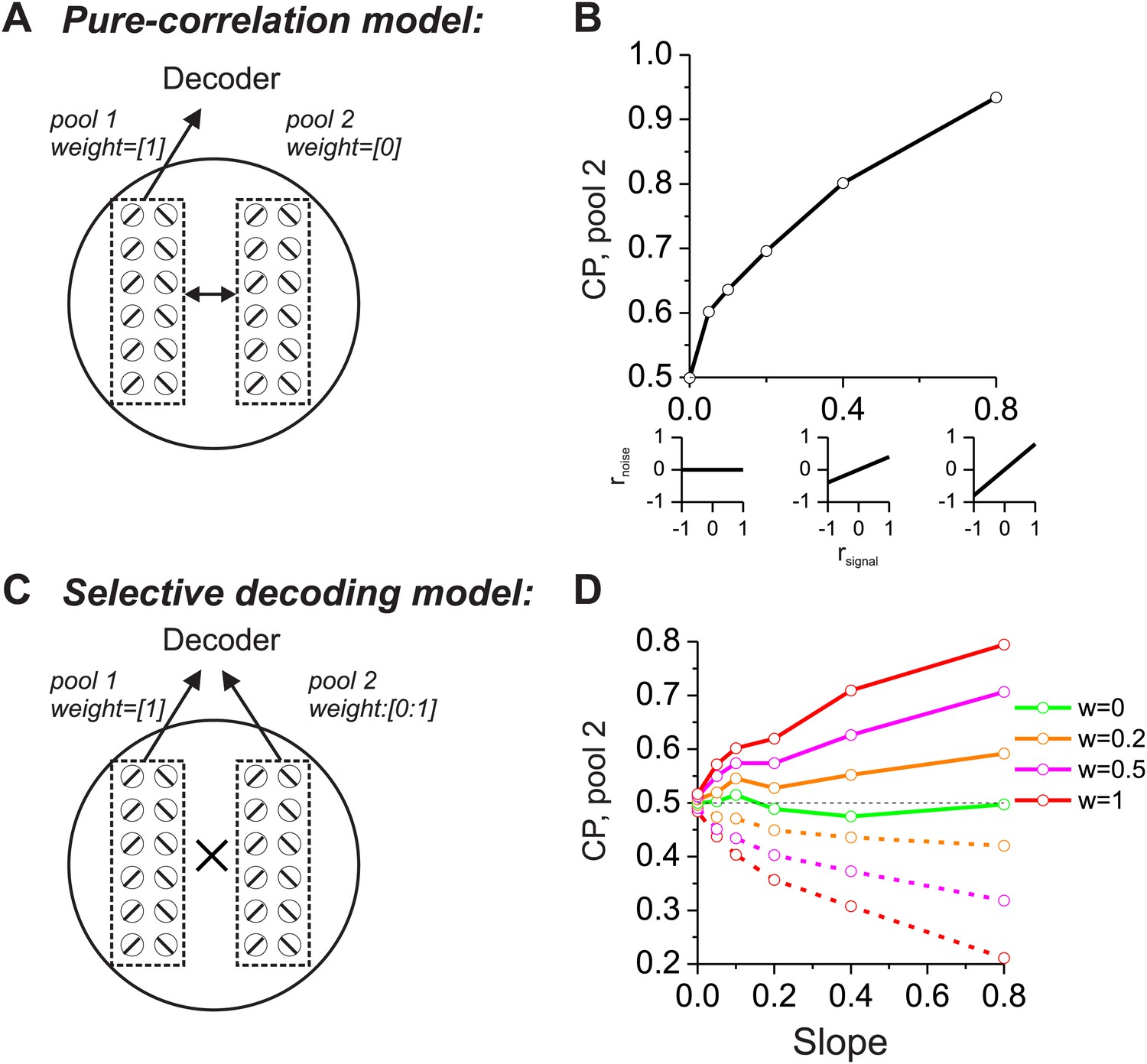
Comparison of models in which choice probabilities (CPs) arise through either correlated noise or selective decoding.
Each model consists of two pools of neurons (500 neurons each) with equal numbers of neurons that prefer leftward and rightward headings. In the 'pure-correlation' model (A and B), neurons in pool 2 make no contribution to the decision and activity within or across pools is correlated according to the relationship illustrated in panel B. In the 'selective decoding' model (C and D), neurons shared correlated noise within each pool but not across pools. Neurons in pool 1 were always given a decoding weight of 1, while neurons in pool 2 were given weights ranging from 0 to 1. Solid curves in D: responses of pool 2 were decoded according to each neuron's preferred stimulus; dashed curves: pool 2 responses were decoded relative to each neuron's anti-preferred stimulus. Dashed black horizontal line: CP = 0.5.
Figure 2 with 3 supplements
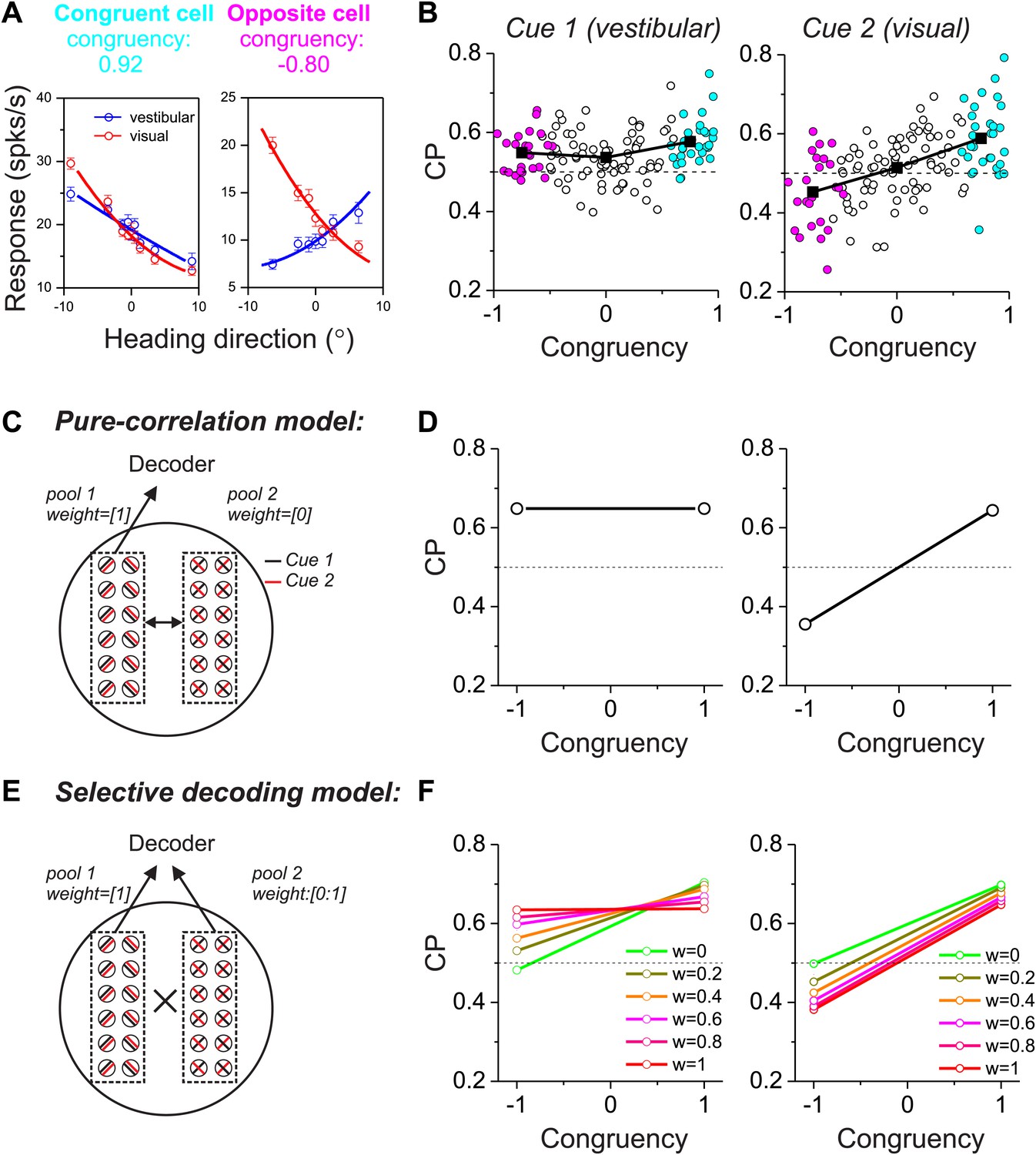
Responses of multisensory neurons and multisensory versions of the pure-correlation and selective-decoding models.
(A) Heading tuning curves from two example MSTd neurons measured during a fine heading discrimination task (Gu et al., 2008): one congruent cell (left) and one opposite cell (right). Red and blue data show responses measured for the visual and vestibular conditions, respectively. (B) Choice probability as a function of congruency for MSTd neurons tested in the vestibular (left) and visual (right) conditions (adapted, with permission, from Supplement Figure 8A and Figure 6C of Gu et al.(2008); respectively). Cyan and magenta symbols denote data for congruent and opposite cells, respectively (unfilled symbols: intermediate cells). (C and D) Multisensory version of the pure-correlation model (500 model neurons in each pool). Pool 1 consists of all congruent cells (same slope tuning curves for the two cues), whereas pool 2 contains all opposite neurons. Correlated noise within or across pools depends only on the similarity of tuning for cue 1. (E and F) In the selective decoding model, neurons were correlated according to the similarity of tuning for both cues (‘Materials and methods’). This rule generated correlated noise within each pool but not between pools. Neurons in pool 1 were always given a full weight of 1 in the decoding, whereas the decoding weights of neurons in pool 2 ranged from 0 to 1 (different colors in F). Dashed black horizontal line: CP = 0.5.
Figure 2—figure supplement 1

Predictions from a variant of the pure-correlation model in which correlated noise depends only on signal correlations from the visual tuning curves.
This modification reverses the patterns of CPs across stimulus conditions, as compared to Figure 2C,D. This pattern of results is not consistent with experimental data.
Figure 2—figure supplement 2
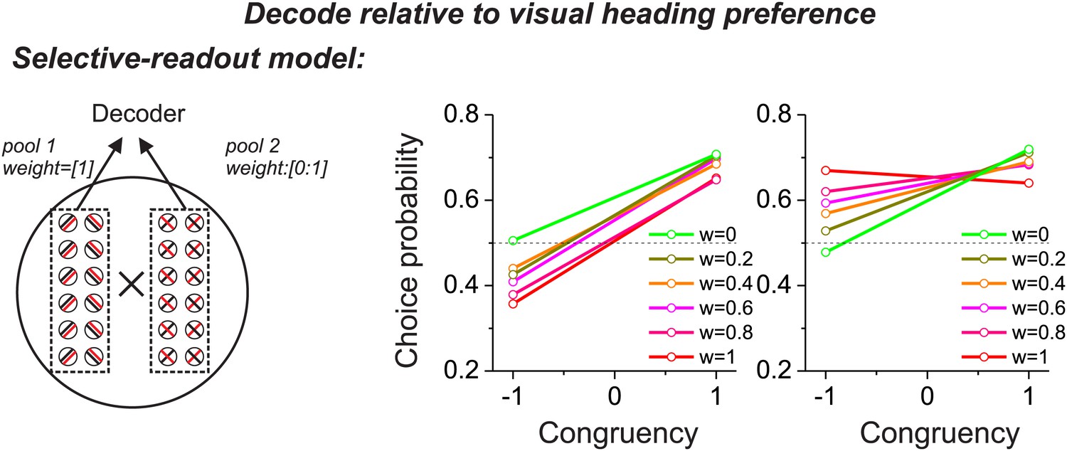
Predictions from a variant of the selective decoding model in which responses are decoded according to the visual heading tuning of each neuron, instead of the vestibular tuning.
This modification reverses the CP patterns across stimulus conditions, as compared to Figure 2E,F, and is inconsistent with experimental data.
Figure 2—figure supplement 3
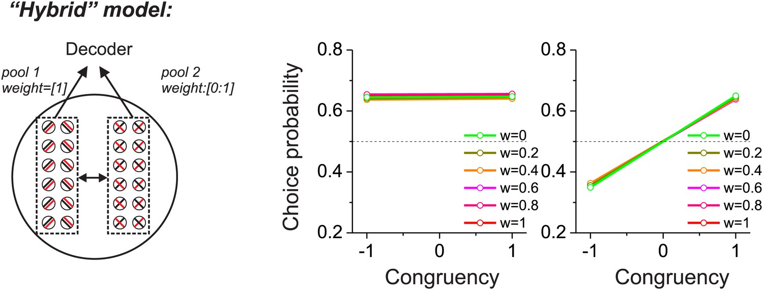
Predictions from a “hybrid” model (see text for details) in which correlated noise was assigned according to vestibular signal correlations, and heading was decoded relative to the vestibular heading tuning of each neuron.
CP patterns were roughly similar to those seen in the pure-correlation model (Figure 2C,D).
Figure 3 with 3 supplements
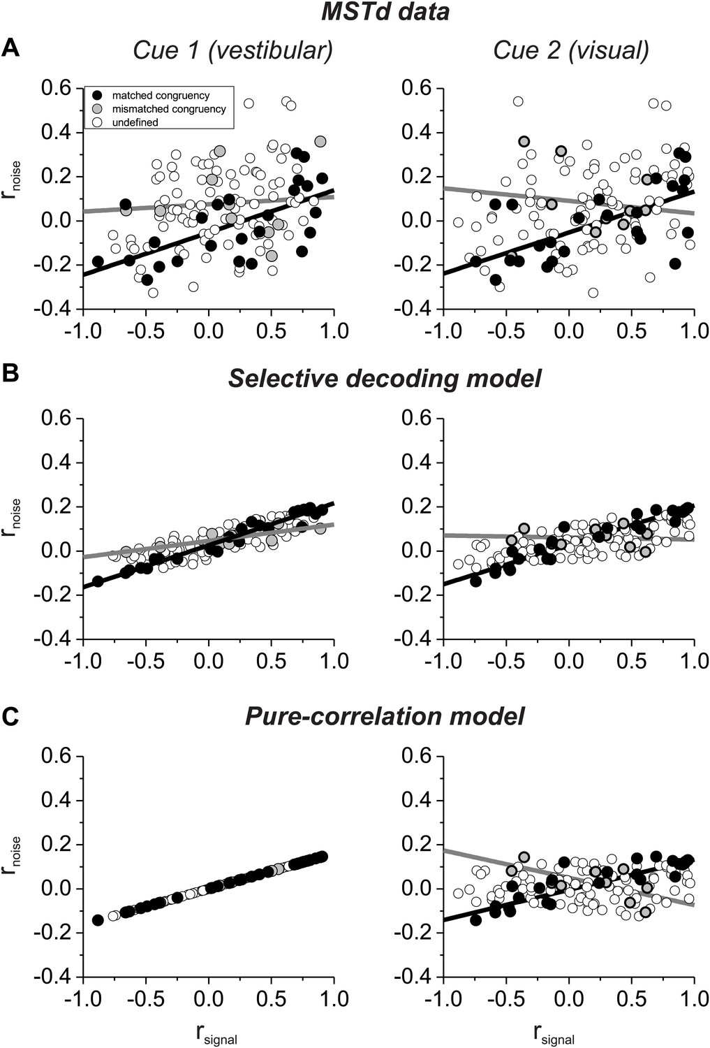
Comparison of the structure of correlated noise between models and data.
(A) Data from pairs of neurons recorded from area MSTd (Gu et al., 2011). Noise correlation is plotted against signal correlations obtained from the vestibular (left column) or visual (right column) tuning curves. Black and gray symbols denote pairs with matched (black) or mismatched (gray) congruency. Open symbols represent undefined pairs. (B) Predicted noise correlations as a function of signal correlation based on fits of the selective decoding model. Format as in panel A. (C) Predicted noise correlations as a function of signal correlation by for the pure-correlation model fit, for which noise correlations depend only on vestibular signal correlation.
Figure 3—figure supplement 1

Comparison of vestibular and visual signal correlations for 127 pairs of neurons simultaneously recorded from area MSTd by Gu et al. (2011).
There is a fairly weak correlation between the two variables (R = 0.29, p=0.001, Spearman correlation). Histograms along the top and right side show marginal distributions of the two signal correlations.
Figure 3—figure supplement 2

Noise correlation structure of the pure correlation model computed from the signal correlations of all distinct pairings of 129 neurons that were recorded previously by Gu et al. (2011).
For the pure-correlation model, correlated noise is determined by the signal correlation in the vestibular condition, such that pairs of cells with matched (black) and mismatched (gray) congruency have opposite relationships between rnoise and rsignal in the visual condition.
Figure 3—figure supplement 3
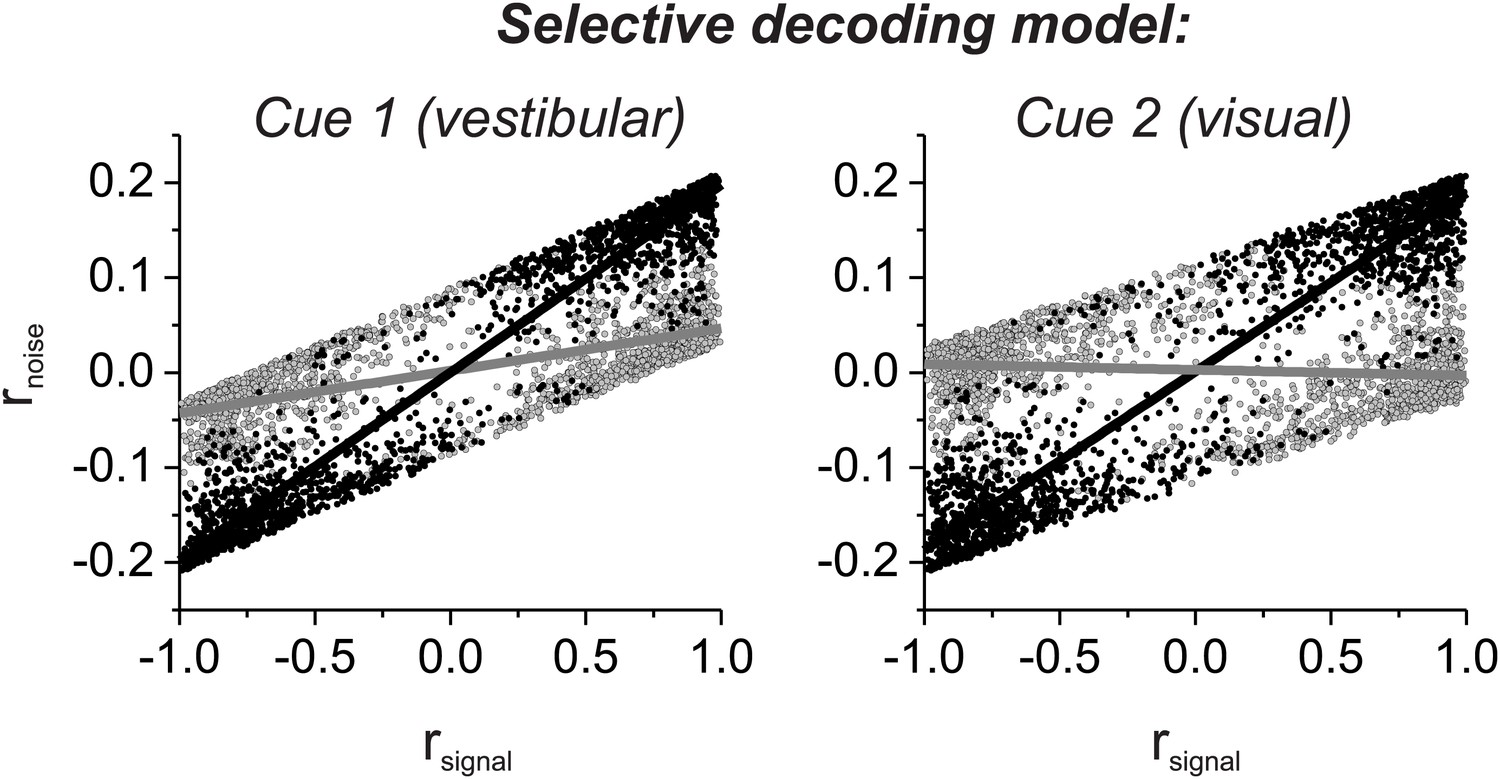
Noise correlation structure of the selective decoding model computed from the signal correlations of all distinct pairings of 129 neurons that were recorded previously by Gu et al. (2011).
For the selective decoding model, correlated noise depends on rsignal in both stimulus conditions. As a result, the relationship between rnoise and rsignal is strong for pairs with matched congruency in both stimulus conditions (black), and this relationship is weak for pairs with mismatched congruency (gray).
Figure 4
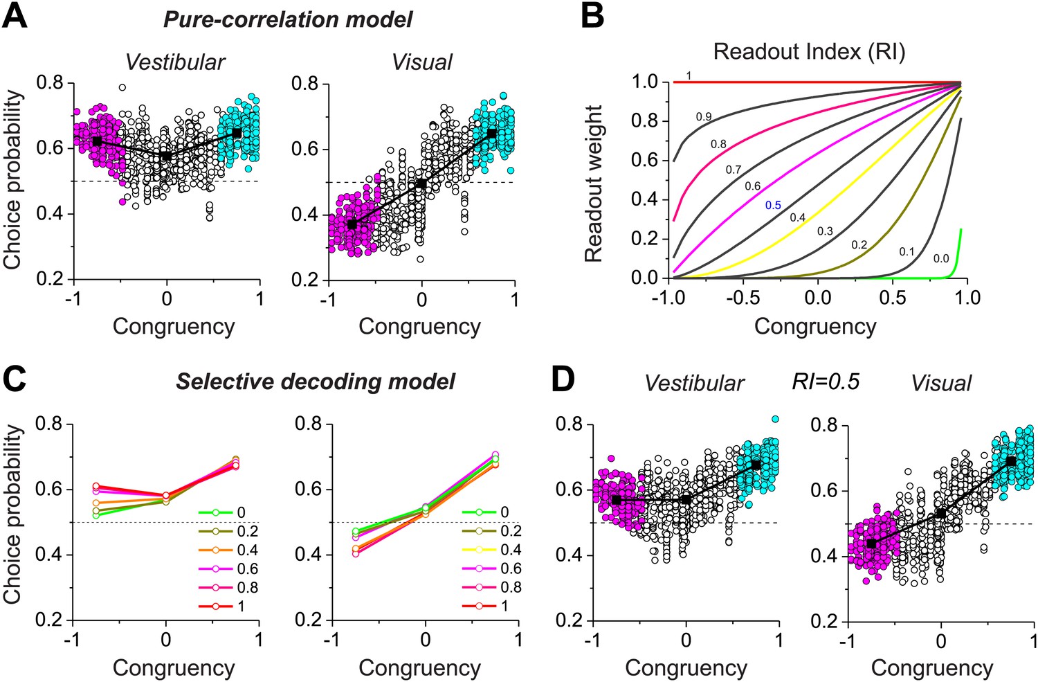
Predictions of choice probabilities from the two models.
(A) The pattern of CPs predicted by the pure-correlation model. Format as in Figure 2B. (B) A family of weighting profiles used to consider various degrees of contribution of opposite cells to the selective decoding model. Each curve shows the decoding weight as a function of congruency between visual and vestibular heading tuning. Each curve corresponds to a specific value of the Readout Index (RI). (C) Predicted average CPs from the selective decoding model for a subset of the RI values illustrated in (B). (D) The pattern of CPs across neurons in the selective decoding model for an RI value of 0.5. Cyan symbols: congruent cells; Magenta symbols: opposite cells; Unfilled symbols: intermediate cells. Solid squares: mean CP. Dashed horizontal line: CP = 0.5.
Figure 5 with 2 supplements
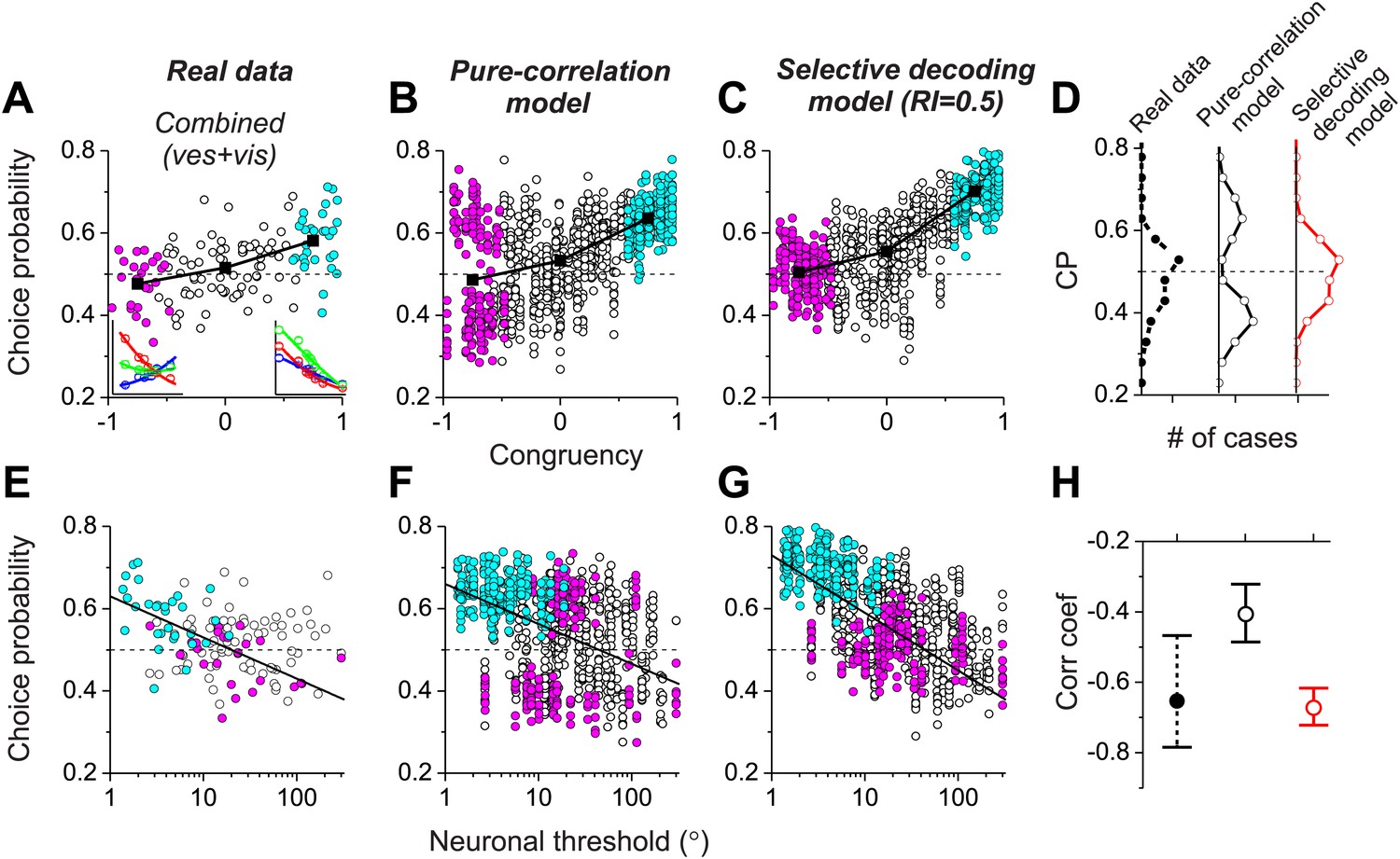
Analysis of choice probabilities for the combined condition in which both visual and vestibular heading cues are present.
(A) CP values plotted as a function of congruency index for neurons from area MSTd tested in the Combined condition (adapted, with permission, from Figure 6A of Gu et al., 2008). (B and C) CP as a function of congruency for model neurons from the pure-correlation model, and model cells from the selective decoding model, respectively. (D) Distributions of CPs for opposite cells from area MSTd, the pure-correlation model and the selective decoding model. (E–G) CP values plotted as a function of neuronal discrimination thresholds for real MSTd neurons (adapted, with permission, from Figure 6B of Gu et al., 2008), units from the pure-correlation model and units from the selective decoding model, respectively. (H) Correlation coefficient of the best linear fit to the relationship between CP and neuronal threshold for MSTd data (filled black circles), pure-correlation model (open black circles) and selective decoding model (open red circles). Error bars represent 95% confidence intervals.
Figure 5—figure supplement 1
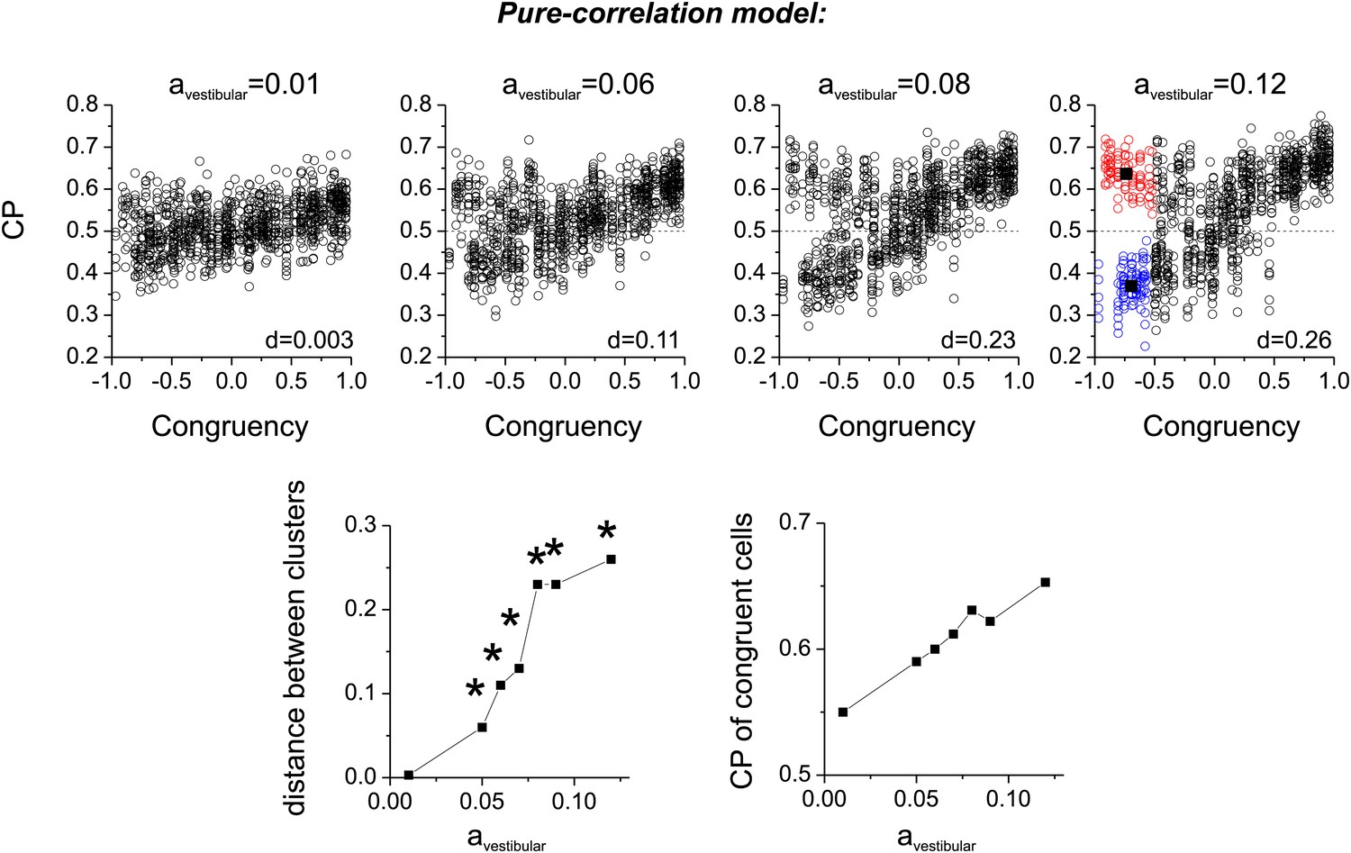
Bimodality of CP for opposite cells in the cue combined condition.
Top panels: four examples of simulations of the pure-correlation model having different values of avestibular ranging from 0.01 to 0.12. Both the magnitude and bimodality of the CP distribution increases with avestibular. To quantify bimodality, we chose cells with Congruency Index in the range [−1–0.5], and applied K-means clustering to generate two clusters. The vertical distance, d, between the centroids of the two clusters was taken as an index of the separation of the two clusters. Bottom row: (left) Summary of d values as a function of avestibular. Asterisks represent significant bimodality, as assessed by a modality test (‘Materials and methods’). (right) Relationship between the CP of congruent cells (congruency index from 0.5 to 1) and avestibular.
Figure 5—figure supplement 2
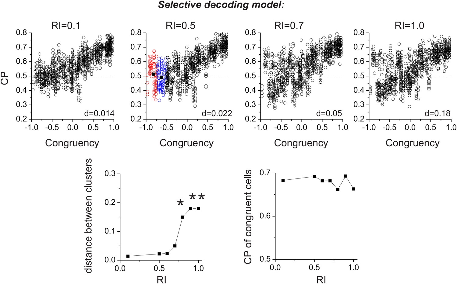
Same format as in Figure 5—figure supplement 1, but results are shown for the selective decoding model.
Top row: simulations for four different values of the Readout Index (RI). Bottom row: A bimodal distribution of CP is only seen for RI values >= 0.8, and CP of congruent cells is independent of RI.
Figure 6 with 1 supplement
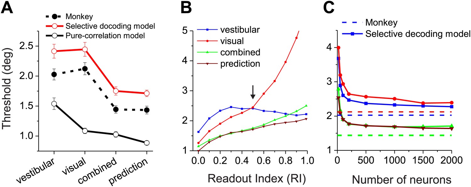
Comparisons between model population threshold and psychophysical performance of the animals.
(A) Average thresholds are shown for the vestibular, visual, and combined conditions, along with the prediction from optimal cue integration theory. Data are shown for the average of two monkeys (filled symbols, dashed curve), for predictions of the pure-correlation model (black open symbols and solid curve), and for predictions of the selective decoding model with RI = 0.5 (red symbols and curve). (B) Predicted thresholds from the selective decoding model are plotted as a function of Readout Index for vestibular, visual, and combined conditions, as well as the optimal prediction from the single-cue thresholds. (C) Thresholds from the selective-decoding model (with RI = 0.5) as a function of population size. Solid curves: model predictions; dashed horizontal lines: average performance of two animals.
Figure 6—figure supplement 1

Comparison of neuronal sensitivity between the visual (ordinate) and vestibular (abscissa) stimulus conditions for 30 congruent cells.
Arrows and numbers indicate geometric mean values. Overall, visual responses were somewhat more sensitive than vestibular responses, although the animals’ behavioral performance was similar between conditions.
Download links
A two-part list of links to download the article, or parts of the article, in various formats.
Downloads (link to download the article as PDF)
Open citations (links to open the citations from this article in various online reference manager services)
Cite this article (links to download the citations from this article in formats compatible with various reference manager tools)
Contribution of correlated noise and selective decoding to choice probability measurements in extrastriate visual cortex
eLife 3:e02670.
https://doi.org/10.7554/eLife.02670


