Reconceiving the hippocampal map as a topological template
- The Jan and Dan Duncan Neurological Research Institute at Texas Children's Hospital, United States
- Baylor College of Medicine, United States
- University of California, San Francisco, United States
Figures
Figure 1 with 1 supplement
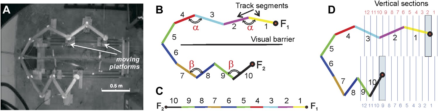
Compressible U/zigzag track (Track A).
(A) Top-down view of the four-meter long track with both arms in a semi-contracted configuration. (B) A schematic representation of the track illustrating how the segments are numbered in the planar (B) and the linear (C) frames of reference. (Note that the track depiction in C is drawn at half the scale as in B. The track was designed so that the angle between the segments 1 and 2 and between segments 3 and 4 on the top arm remain the same whether the track arm is extended or compressed, that is, ∠(1,2) = ∠(3,4) = α. Similarly, the angles on the bottom arm remain equal, ∠(7,8) = ∠(9,10) = β. The magnitude of angle α is defined by the stretch of the top arm (by the position of the food well F1), and angle β is defined by the position of the food well F2. Thus, the geometric configuration of the track can be described either by the angles (α, β) or the positions of the food wells F1 and F2. (D) To more readily denote track arm configurations, we divided the space that can be occupied by the fully extended top and bottom arms into 12 vertical sections each. Each position of a track arm can be described by the numbered vertical section into which F1 or F2 (for the top and bottom arms, respectively) falls. In the depicted track configuration, F1 falls into section 2 and F2 falls into section 9. However, because we are interested in being able to denote changes in track segment positions in order to compute correlation coefficients, the top arm can be said to move from position i to position j (numbers in red), and the bottom arm from position k to position l (numbers in blue; see ‘Materials and methods’). So the track configuration depicted here can be fully described by F1 = 2 and F2 = 9. Given movement of an arm from section i to j (or k to l), the larger the difference between the numbers, d=|i − j | or |k − l|, the more geometrically dissimilar positions i and j or k and l are.
Figure 1—figure supplement.1
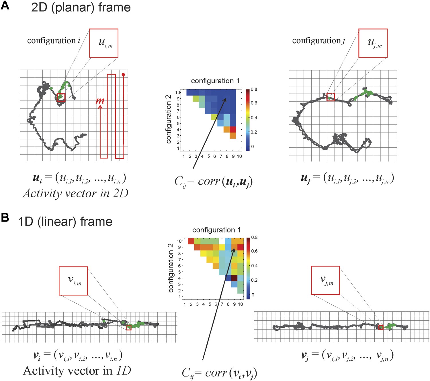
Calculating correlation coefficients for place cells firing in different track configurations.
The grid covering the 2D space occupied by the track is binned into squares that are 3 cm × 3 cm. The red line illustrates how we sequenced the bins in the planar and linear reference frames, with m = 1 at the top right square, m = 2 the square below it, etc. The activity vector ui or uj is the firing rate of a place cell given a particular track configuration (i on the left, j on the right, respectively) in the 2D frame of reference and is constituted by the firing rates of the cell in particular bins (ui1, ui2, etc). In the example in panel A, the same spatial bin produces vector components ui,m (in configuration i) and uj,m (in track configuration j). We calculate the correlation coefficient, Ci,j, to understand the relationship between two activity vectors for a given place cell firing in two different track configurations (for the sake of simplicity, we depict only a change of position in the top arm, from i to j; we can do this safely because the place cells we recorded did not have multiple place fields). Note that any given configuration can be arrived at from a number of movements: the top arm could move to position 2 from vertical sections 1 or 3, 7, or 10 (see Figure 1D), so the correlation coefficient for a cell that has a place field on the top arm, Ci,j would be denoted by C1,2, C3,2, C7,2, or C10,2, respectively. As explained in Figure 1D, the greater the numeric difference between i and j, the greater the geometric difference between track configurations 1 and 2. The correlation matrix in the middle graphically depicts correlation coefficients by color. In panel B we show activity vectors vi, vj for linearized trajectories of the animal along the same configurations i and j depicted in 2D in panel A.
Figure 2
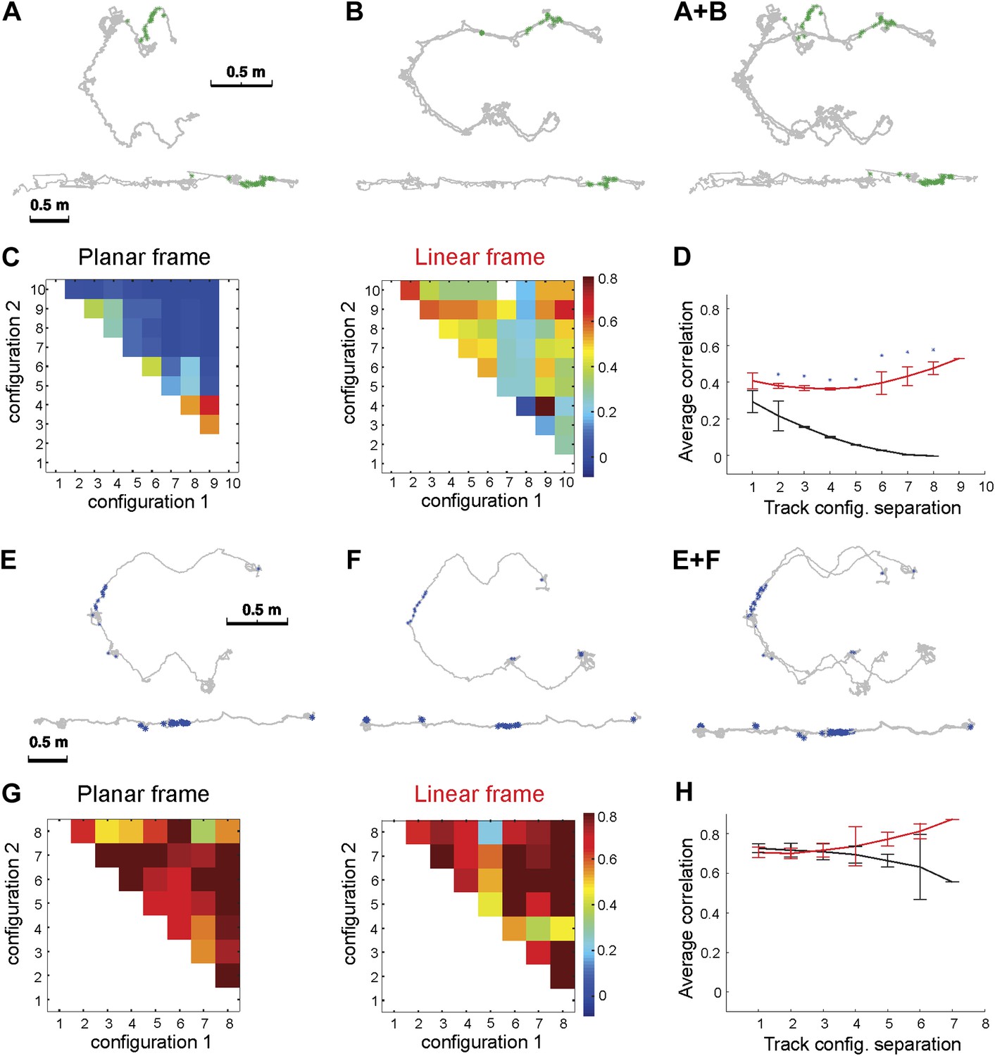
Place cell spiking across different configurations of Track A shows that place fields remain stable despite large geometric changes.
Depicted are the firing patterns of two place cells: one cell that was active primarily on one dynamic segment of the track (A–D) and another place cell that was active on a static part of the track (E–H). (A) Each green dot represents a spike, which is shown in two reference frames: 2D (upper row) and linear (bottom row). The gray line represents the animal's path across all trials with these configurations. (B) Overlaying the 2D and linear reference frames shows that the spiking is distributed in 2D space but much more localized in the linearized reference frame. (C) The matrix of the correlations between the activity of this place cell over the moving sections of the track defined in planar (left) and in the linear (right) frame. The color of each square (Cij) represents the mean correlation coefficient between two track configurations, configuration1 and configuration2. The correlations were clearly much higher in the linear frame. (D) The mean correlation coefficient values, rd = < Ci,i+d >, averaged over all pairs of the track configurations separated by d bins. The lines show whether the place cell firing was stable across configurations in the linear (1D, red) and the planar (2D, black) reference frames as a function of the difference d between the two configurations; the black line shows clear decay of correlation between the configurations, meaning that place cell firing was not stable in 2D (See Figure 1 for explanation of D). (E–H) The same plots for a different neuron (spikes shown in blue) that was active on the static track segments. The graph to the right shows a high correlation coefficient for both frames of reference, indicating that the place fields were stable. The asterisk above the SEM error bars indicates p < 0.001. A total of 557 neurons were recorded; the place cells depicted here are representative.
Figure 3
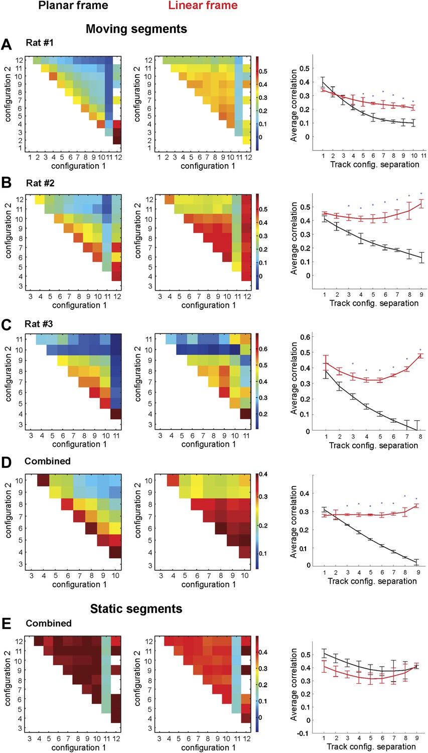
Place cell firing is stable across different track configurations.
(A–C) The correlograms for the ensemble averages for each of three animals. The place cell spiking data are taken from only the segments of the track that change position between configurations. The two lines on the graphs in the third column represent the correlation coefficients of place cell ensembles in the 1D (red) and 2D (black) frames of reference. The correlation coefficients in the 1D configuration (red lines) remain stable, but the correlation coefficients for the 2D configuration (black lines) decay as the geometric difference between track configurations increases. (D) Combined data from all three rats for the correlation coefficients for the combined ensemble averages over all mobile track segments. Only data from the moving segments of the track and the corresponding correlations vs track configuration separation plot for the two reference frames are included. Firing across the population was much more stable in the linear reference frame. (E) The same plots as in D for spikes fired over the static sections of the track. Error bars represent SEM and * indicates p < 0.001.
Figure 4
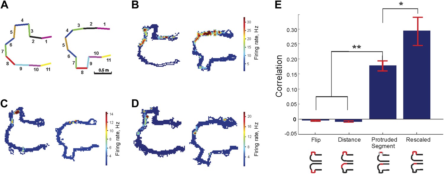
Protrusion-flip track (Track B).
(A) Schematic representation of Track B, with segments numbered, showing the position of the track's protrusion during two successive run sessions. (B–D) Each show a representative place cell firing in the two configurations. (E) Correlations for each of the four comparisons of regions across the two configurations. The rescaled correlation is highest, indicating that the data are most compatible with a scheme in which the place cell firing does not simply respond to changes in geometry. Error bars represent SEM with * and ** indicating p < 10−8 and < 10−9 , respectively.
Author response image 1
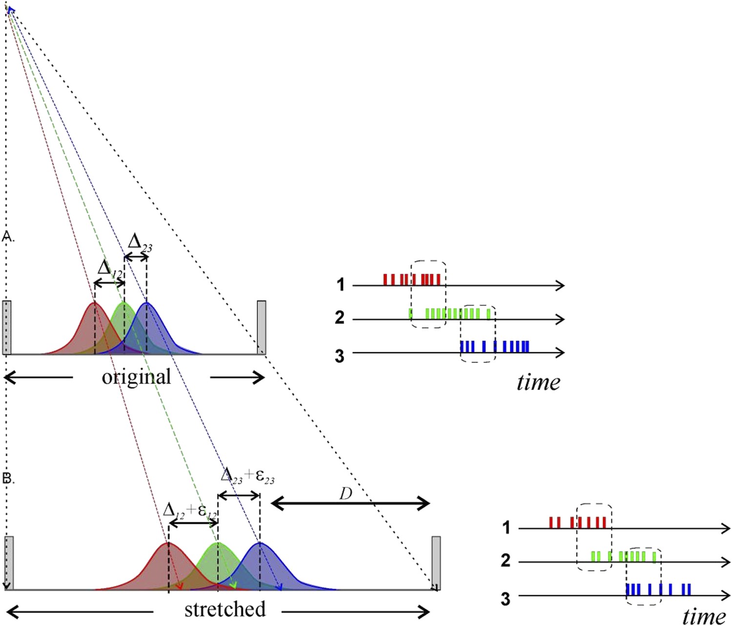
Metrical information contained in stretching place fields will not necessarily be conveyed by place cell spiking to downstream neurons. A) Three place fields (red, green and blue) stretch following the enlargement of the enclosure. To the right we show how the overlap between the place fields reflects the pattern of temporal overlap between the place cell’s spike trains; the rate of coactivity events depends on the distance between the place field centers, Δij = ri − rj, where ri is the distance of the ith place field from the track’s center, their widths and the spiking rate amplitudes. B) After the environment expands over the distance D, the place fields’ layout stretches and the fields’ centers shift proportionally to their distances from the walls of the enclosure (Diba and Buzsaki, 2008; Gothard et al., 1996). According to (O'Keefe and Burgess, 1996), some place fields may even remain at a fixed distance from the walls of the enclosure. In either case, the change in the distance between the place field centers is small. For example, consider two place fields on a 1-meter-long track located at r1 = 50 cm and r2 =60 cm, respectively. After the track stretches over D =100 cm, the place fields will move to r′1 = 100 cm and r′2 = 120 cm. As a result, if the original distance between place fields was Δ12 = 10 cm, after the stretch it will be Δ′12 =20 cm. The increase in distance between place field centers is thus only ε12 =10 cm, or 10% of the full stretch. Since place cell activity is modulated by an animal’s speed, visual cues, odor, and a plethora of other factors, a particular readout neuron would have no way of determining whether the change in firing rate is due to a geometric determinant, the animal slowing down, a change in a visual cue, or something else. Thus, even if the place field layout stretches significantly, the corresponding geometrical information would not necessarily be captured by the downstream networks unless the change is quite large.
Download links
A two-part list of links to download the article, or parts of the article, in various formats.
Downloads (link to download the article as PDF)
Open citations (links to open the citations from this article in various online reference manager services)
Cite this article (links to download the citations from this article in formats compatible with various reference manager tools)
Reconceiving the hippocampal map as a topological template
eLife 3:e03476.
https://doi.org/10.7554/eLife.03476


