Neural mechanisms of economic commitment in the human medial prefrontal cortex
Figures

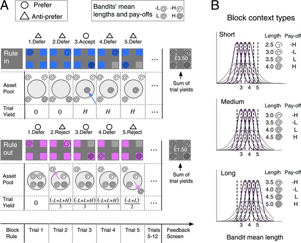
Block timeline and task design.
(A) Upper left inset box: in the two examples, preference and anti-preference for a bandit is indicated with an open circle and triangle, respectively. Upper right inset box: showing the mapping between mean spiral length and payoff (H for high and L for low) of the four bandits in the example blocks. Upper panel: example of a rule-in block. Following an instruction screen, on each trial (grey panels) four bandits (colored boxes) were presented. A spiral in one box provided a noisy estimate of bandit mean length. Bandits that were accepted were made unavailable (greyed out) for future choices (trial 4). Accepted bandits were brought irrevocably into a virtual ‘asset pool’ (light gray circle) that began empty (trial 3). The per-trial yield, that is, the average of the payoffs of all bandits in the asset pool, was aggregated to provide the block-end yield. After 12 trials a feedback screen revealed each bandit’s nominal length and winnings. Bottom panel: same as upper, but for a rule-out block. All bandits began in the asset pool. Rejection eliminated one bandit from the pool (trials 2 and 5). Per-trial yield reflected the average payoff of bandits not yet eliminated from the asset pool. (B) The bandits’ length distributions could vary across 2-variance level (purple/grey). Payoff reflected the rank order of a bandit‘s mean spiral length within the block. The average mean length of the 4 bandits ranged from 2.5 to 5 (see ‘Materials and methods’) and was manipulated across 3 levels corresponding to three different context types.

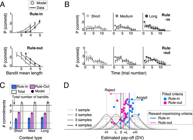
Behavioral results (N = 20) and model predictions.
(A) Commitment probability in different contexts (short, medium and long blocks) as a function of mean bandit spiral length for rule-in (top) and rule-out blocks (bottom) and (B) probability of commitment as a function of trial number, context-type and rule. Black lines: human data; filled gray circles: model fits. (C) Mean number of commitments in rule-in and rule-out (and their sum), in the three different contexts. Moving from short to long contexts, commitments increased in rule-in (F(2,38) = 6.73, p < 0.01) and decreased in rule-out (F(2,38) = 4.95, p < 0.05). The model predicts this pattern (filled circles) by initializing the block reference to the mean spiral length in the experiment (see ‘Materials and methods’), thus over(under)-estimating the DV at trial 1 in long (short) contexts. The sum of commitments exceeded the number of available bandits (4.5 ± 0.6; t(19) = 3.64, p < 0.005), mainly due to more than one commitments made in rule-in. (D) Fitted decision criteria (filled circles) did not significantly differ from reward-maximizing criteria (solid vertical lines) under the current-minus-average model for rule-in (blue) and rule-out (purple). Gray curves show the distributions of the estimated pay-off for each of the four bandits under different numbers of samples (different shades). Values larger (smaller) than the rule-in criterion provoke inclusion by commitment (exclusion by deferral). Values smaller (larger) than the rule-out criterion result in exclusion by commitment (inclusion by deferral). Bars are 95% confidence intervals (C.I.). H and L stand for bandits with high and low absolute pay-off, respectively.

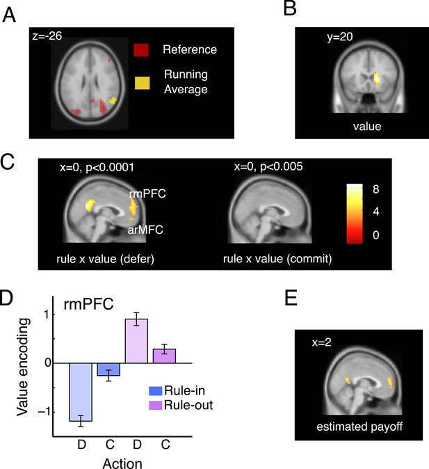
Imaging data: model validation and rmPFC.
(A). Overlapping activations in the parietal cortex elicited by the current bandit running average (yellow; peak: 58, −60, 26; t(19) = 4.78, p < 0.0002) and reference (red; peak: 34, −68, 22; t(19) = 6.17, p < 0.00001). (B) In the right caudate nucleus, we also observed a representation of the difference between these two quantities, that is, voxels that co-varied with the DVcur − ave but did not vary according to the rule type or decision (main effect of the value signal; peak: 18, 20, 2; t(19) = 6.63, p < 0.00001). (C) Voxels responding to the interaction of rule and value on defer trials (left, at p < 0.0001) and commit trials (right, at p < 0.001). Value is encoded (in the frame of reference of the rule) only on defer trials. (D) Mean parameter estimates, derived by regressing bandit value on the BOLD signal from within an independently-defined ROI in the rmPFC, separately for defer and commit decision under each rule. To ensure independence, ROIs were defined individually for each participant as the peak voxel responding within the region in the remaining 19 participants. All significant voxels are visualized at p < 0.001 and survive correction for multiple comparisons across the brain. (E) Parameter estimates from a regressor encoding the value of the asset pool (estimated final payoff).

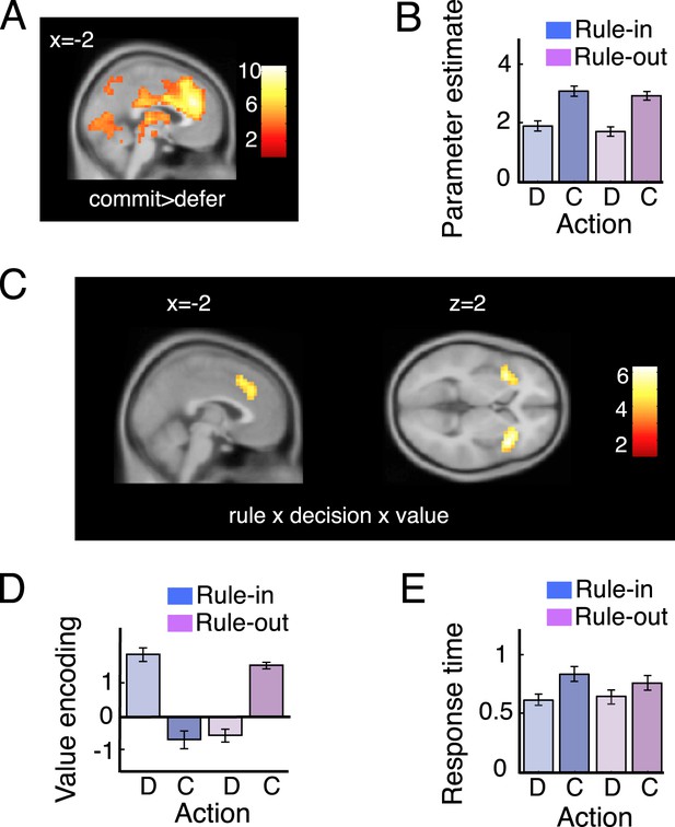
Imaging data: dACC.
(A) Voxels responding to commit > defer, rendered onto a sagittal slice of a template brain (see also Figure 4—source data 1). The red-white scale shows t-values. (B) Average BOLD responses for defer (D) and commit (C) trials on rule-in (blue) and rule-out (magenta) blocks. (C) Voxels responding to the three-way interaction of rule, decision and value, in the ACC. (D) Bar plots showing average parameter estimates for a regression of value on BOLD activity in regions of interest (ROI) in the ACC, separately for defer and commit decision under each rule. Legend as for 3D. (E) Response times (seconds) were overall slower during commitment and this difference was pronounced in rule-in trials. This pattern is comparable with ACC average bold for defer and commit (B). Error bars are 95% confidence intervals (C.I.).
-
Figure 4—source data 1
Local maxima responding to commit > pass, at a FWE-corrected threshold of p < 0.05.
Columns show cluster and peak statistics as well as the x, y, z coordinates of the peaks.
- https://doi.org/10.7554/eLife.03701.008
Tables
Negative log-likelihood (−LL; mean and standard deviation) for the eight decision variables, combing differently anchoring and integration processes
| Anchor | Integration | ||||
|---|---|---|---|---|---|
| No | Yes | ||||
| r(t) | DV(t) | −LL | DV(t) | −LL | |
| No | N/A | si(t) | 200 ± 25 | 195 ± 26 | |
| Previous | sj(t − 1) | si(t) − r(t) | 211 ± 24 | 208 ± 23 | |
| Max-next | si(t) − r(t) | 183 ± 24 | 178 ± 25 | ||
| Average | si(t) − r(t) | 189 ± 23 | 167 ± 28 | ||
-
The best fitting DV (Anchor: average, Integration: Yes) is highlighted with bold. We refer to this DV in the text as current-minus-average. The second best DV (Anchor: Max-next, Integration: Yes) is mentioned in the text as current-minus-next.


