Variance predicts salience in central sensory processing
- University of Pennsylvania, United States
- École Normale Supérieure, France
- Weill Cornell Medical College, United States
- City University of New York Graduate Center, United States
- Institute of Science and Technology Austria, Austria
Figures
Figure 1 with 3 supplements
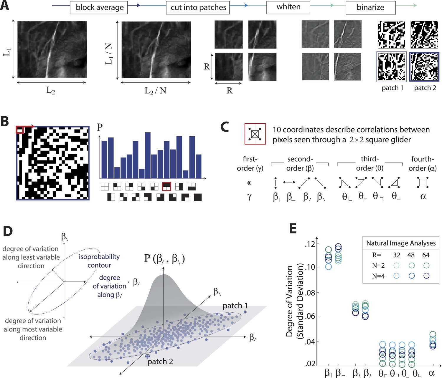
Extracting image statistics from natural scenes.
(A) We first block-average each image over N × N pixel squares, then divide it into patches of size R × R pixels, then whiten the ensemble of patches by removing the average pairwise structure, and finally binarize each patch about its median intensity value (see ‘Materials and methods’, Image preprocessing). (B) From each binary patch, we measure the occurrence probability of the 16 possible colorings as seen through a two-by-two pixel glider (red). Translation invariance imposes constraints between the probabilities that reduce the number of degrees of freedom to 10. (C) A convenient coordinate basis for these 10° of freedom can be described in terms of correlations between pixels as seen through the glider. These consist of one first-order coordinate (γ), four second-order coordinates (), four third-order coordinates (), and one fourth-order coordinate (α). Since the images are binary, with black = −1 and white = +1, these correlations are sums and differences of the 16 probabilities that form the histogram in panel B (Victor and Conte, 2012). (D) Each patch is assigned a vector of coordinate values that describes the histogram shown in (B). This coordinate vector defines a specific location in the multidimensional space of image statistics. The ensemble of patches is then described by the probability distribution of coordinate values. We compute the degree of variation (standard deviation) along different directions within this distribution (inset). (E) Along single coordinate axes, we find that the degree of variation is rank-ordered as , shown separately for different choices of the block-average factor N and patch size R used during image preprocessing.
Figure 1—figure supplement 1
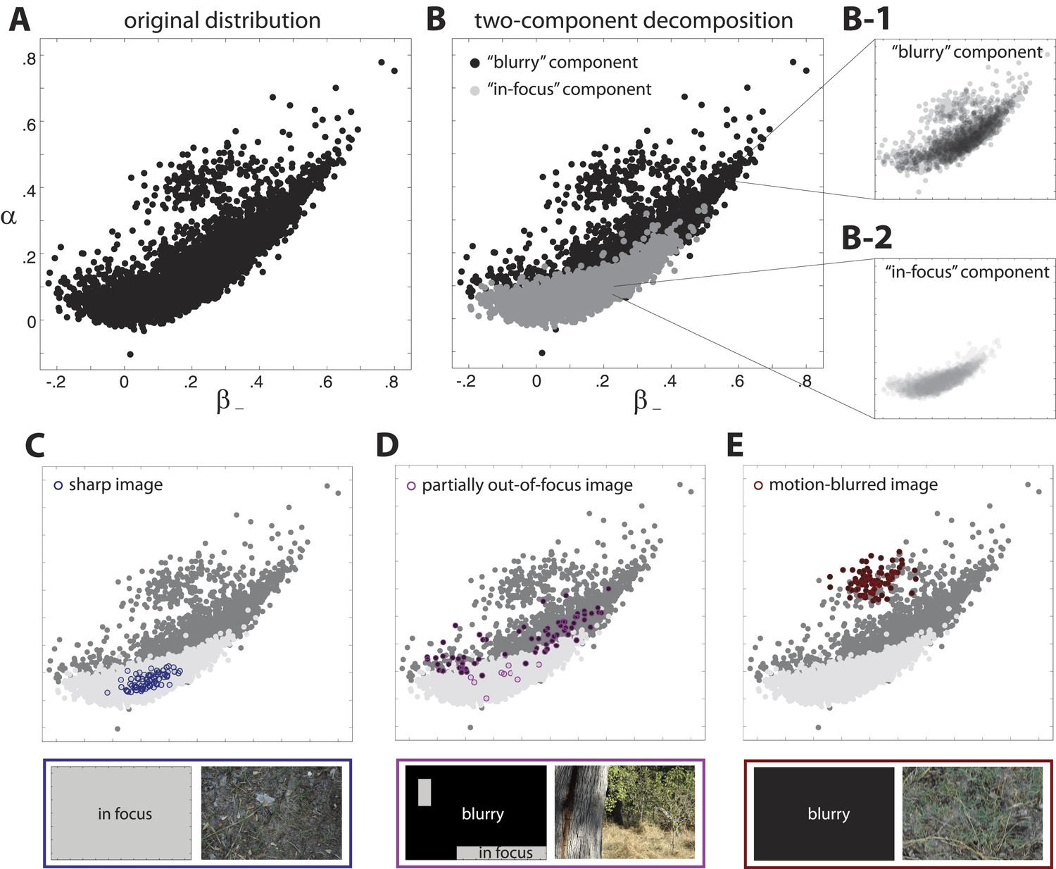
Two-component decomposition of natural image distribution.
(A) The 9-dimensional distribution of natural image statistics is shown projected onto the plane, where each point represents a single image patch. Note that it is not possible to see all points in the distribution due to their overlap. (B) This distribution is well described by a mixture of two components in which each image patch is assigned to one of the two components. Inspection of the image patches assigned to each component reveals that one component (light gray) contains in-focus patches, while the other component (black) contains blurred patches. Note that the two components are separated in the full 9-dimensional space but appear overlapping when projected onto a single coordinate plane. Insets show semi-transparent versions of the out-of-focus B-1 and in-focus (B-2 components. We highlight the coordinate values of specific images that are C fully in focus, (D) blurred due to variations in field of depth, and (E) blurred due to camera motion. Spatial distributions of patch assignments (left) and original image patches (right) are shown below each distribution. (C) A sharp image is composed of patches that are uniformly assigned to the ‘in-focus’ component. (D) An image that is partially out of focus due to variations in field of depth has patches that are assigned to each of the two components. (E) An image that is blurred due to camera motion is composed of patches that are uniformly assigned to the “blurry” component.
Figure 1—figure supplement 2
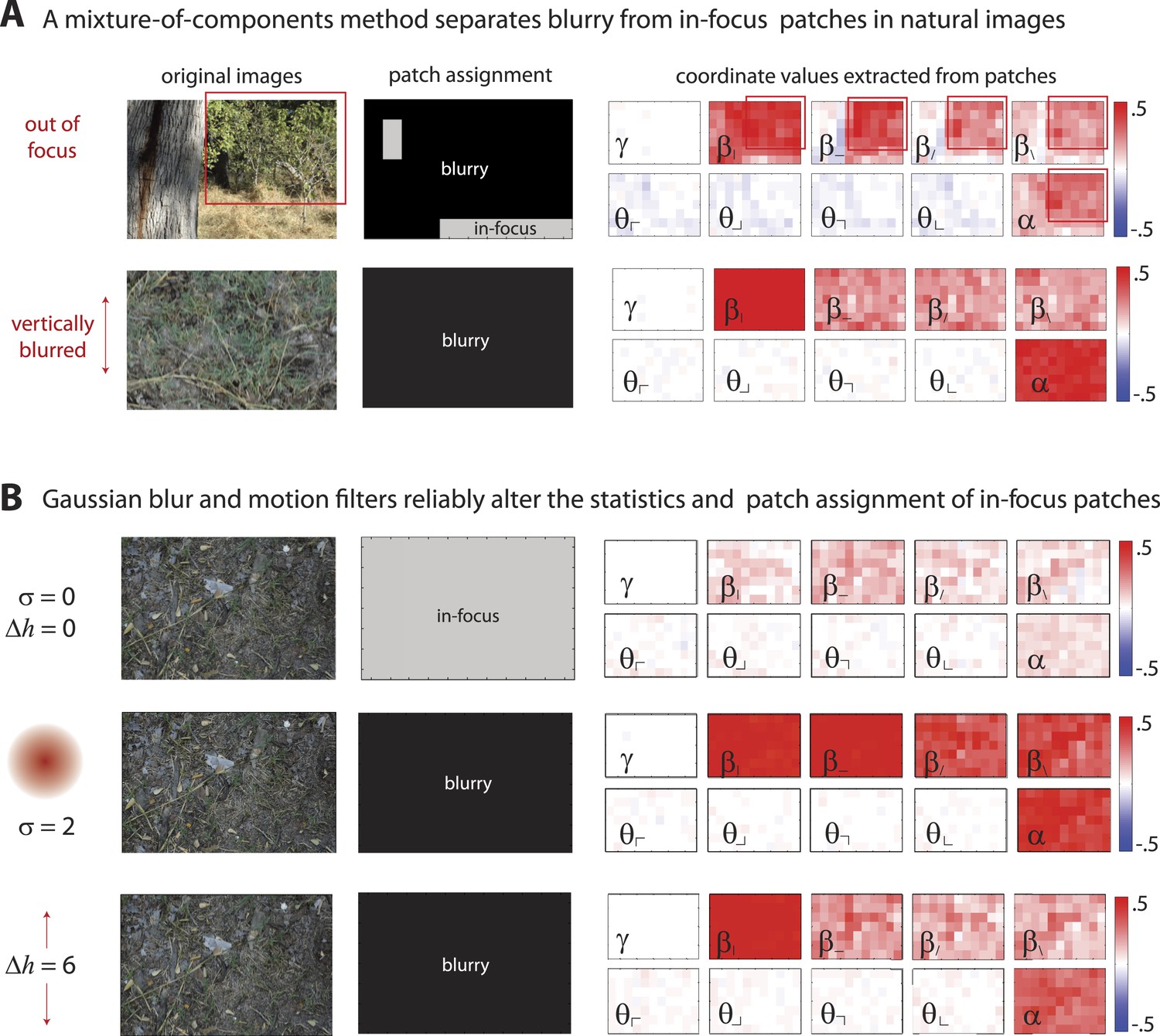
Filtering via defocus or motion blur reassigns sharp image patches to the ‘blurry’ component.
(A) Images can be blurred due to variations in field of depth (upper row) or camera motion (lower row). A mixture of components (MOC) method separates blurry (black) from in-focus (gray) image patches. Patches assigned to the ‘blurry’ component have larger positive coordinate values (red), showing saturated values of second- and fourth-order coordinates. Blurring due to variations in field of depth tends to uniformly increase all second- and fourth-order statistics. In comparison, motion blurring tends to more strongly increase both the fourth-order statistic and the second-order statistic aligned with the direction of motion (here, ). (B) The application of a Gaussian blur filter (middle row) or a motion filter (bottom row) to an in-focus image (top row) produces similar effects; with a sufficiently strong filter (Gaussian blur of pixels or motion of pixels), all patches in the original ‘in-focus’ image are reassigned to the ‘blurry’ component. Furthermore, both the Gaussian blur and motion filters alter the distribution of image statistics in a consistent manner. Gaussian blur filters increase the values of all second- and fourth-order coordinates, while motion filters more strongly increase the values of the fourth-order coordinate and the second-order coordinate aligned with the direction of motion.
Figure 1—figure supplement 3
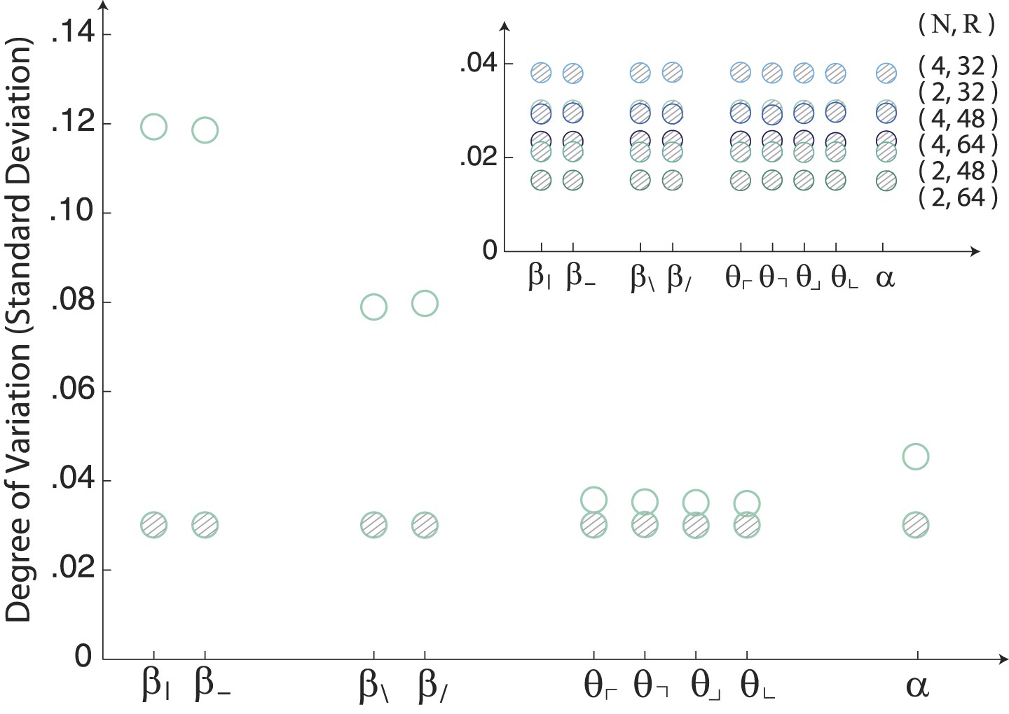
Image statistics along single coordinate axes for white-noise patches.
The robustly observed statistical structure of natural scenes (open circles) is completely absent from the same analysis performed on samples of white noise (shaded circles). The inset shows that this holds across analysis parameters.
Figure 2
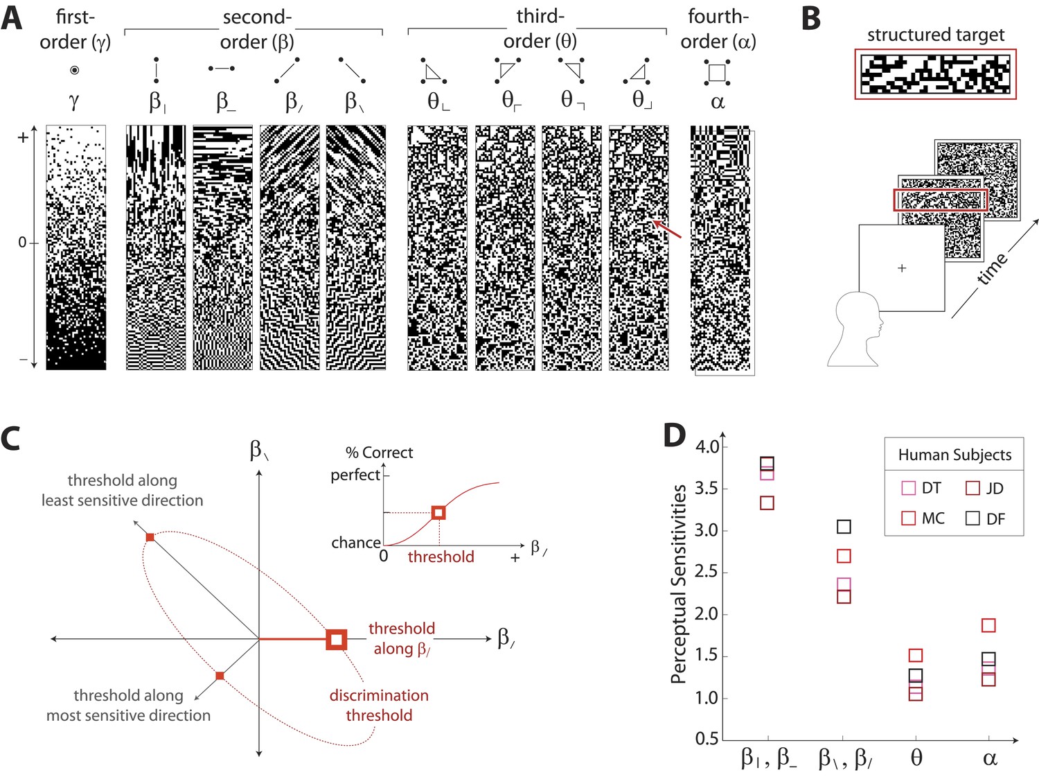
Measuring human sensitivity to image statistics.
(A) Synthetic binary images can be created that contain specified values of individual image statistic coordinates (as shown here) or specified values of pairs of coordinates (Victor and Conte, 2012). (B) To measure human sensitivity to image statistics, we generate synthetic textures with prescribed coordinate values but no additional statistical structure, and we use these synthetic textures in a figure/ground segmentation task (See Victor and Conte, 2012 and ‘Materials and methods’, Psychophysical methods). (C) For measurements along coordinate axes, test stimuli are built out of homogeneous samples drawn from the gamuts shown in A (e.g. the target shown in B was generated from the portion of the gamut indicated by the red arrow in A; See ‘Materials and methods’, Psychophysical methods, and Victor et al., 2005; Victor and Conte, 2012; Victor et al., 2013). We assess the discriminability of these stimuli from white noise by measuring the threshold value of a coordinate required to achieve performance halfway between chance and perfect (inset). A similar approach is used to measure sensitivity in oblique directions; here, two coordinate values are specified to create the test stimuli. The threshold values along the axes and in oblique directions define an isodiscrimination contour (red dashed ellipse, main panel) in pairwise coordinate planes. (D) Along individual coordinate axes, we find that sensitivities (1/thresholds) are rank-ordered as , shown separately for four individual subjects. A single set of perceptual sensitivities is shown for , , and , since human subjects are equally sensitive to rotationally-equivalent pairs of second-order coordinates and to all third-order coordinates (Victor et al., 2013).
Figure 3 with 9 supplements
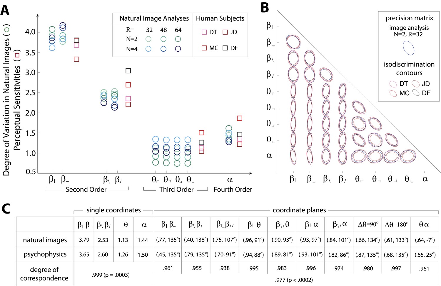
Variation in natural images predicts human perceptual sensitivity.
(A) Scaled degree of variation (standard deviation) in natural image statistics along second- (β), third- (θ), and fourth-order (α) coordinate axes (blue circular markers) are shown in comparison to human perceptual sensitivities measured along the same coordinate axes (red square markers). Degree of variation in natural image statistics is separately shown for different choices of the block-average factor (N) and patch size (R) used during image preprocessing. Perceptual sensitivities are separately shown for four individual subjects. As in Figure 2C,A single set of perceptual sensitivities is shown for , , and . (B) For each pair of coordinates, we compare the precision matrix (blue ellipses) extracted from natural scenes (using N = 2, R = 32) to human perceptual isodiscrimination contours (red ellipses). Coordinate planes are organized into a grid. The set of ellipses in each pairwise plane is scaled to maximally fill each portion of the grid; agreement between the variation along single coordinate axes and the corresponding human sensitivities (shown in A) guarantees that no information is lost by scaling. Across all 36 coordinate planes, there is a correspondence in the shape, size, and orientation of precision matrix contours and perceptual isodiscrimination contours. (C) Quantitative comparison of a single image analysis (N = 2, R = 32) with the subject-averaged psychophysical data. For single coordinates depicted in A, we report the standard deviation in natural image statistics (upper row) and perceptual sensitivities (middle row). For sets of coordinate planes depicted in (B), we report the (average eccentricity, angular tilt) of precision matrix contours from natural scenes (upper row) and isodiscrimination contours from psychophysical measurements (middle row). The degree of correspondence between predictions derived from natural image data and the psychophysical measurements can be conveniently summarized as a scalar product (see text), where 1 indicates a perfect match. In all cases, the correspondence is very high (0.938–0.999) and is highly statistically significant (p ≤ 0.0003 for both single coordinates and pairwise coordinate planes; see ‘Materials and methods’, Permutation tests, for details).
Figure 3—figure supplement 1
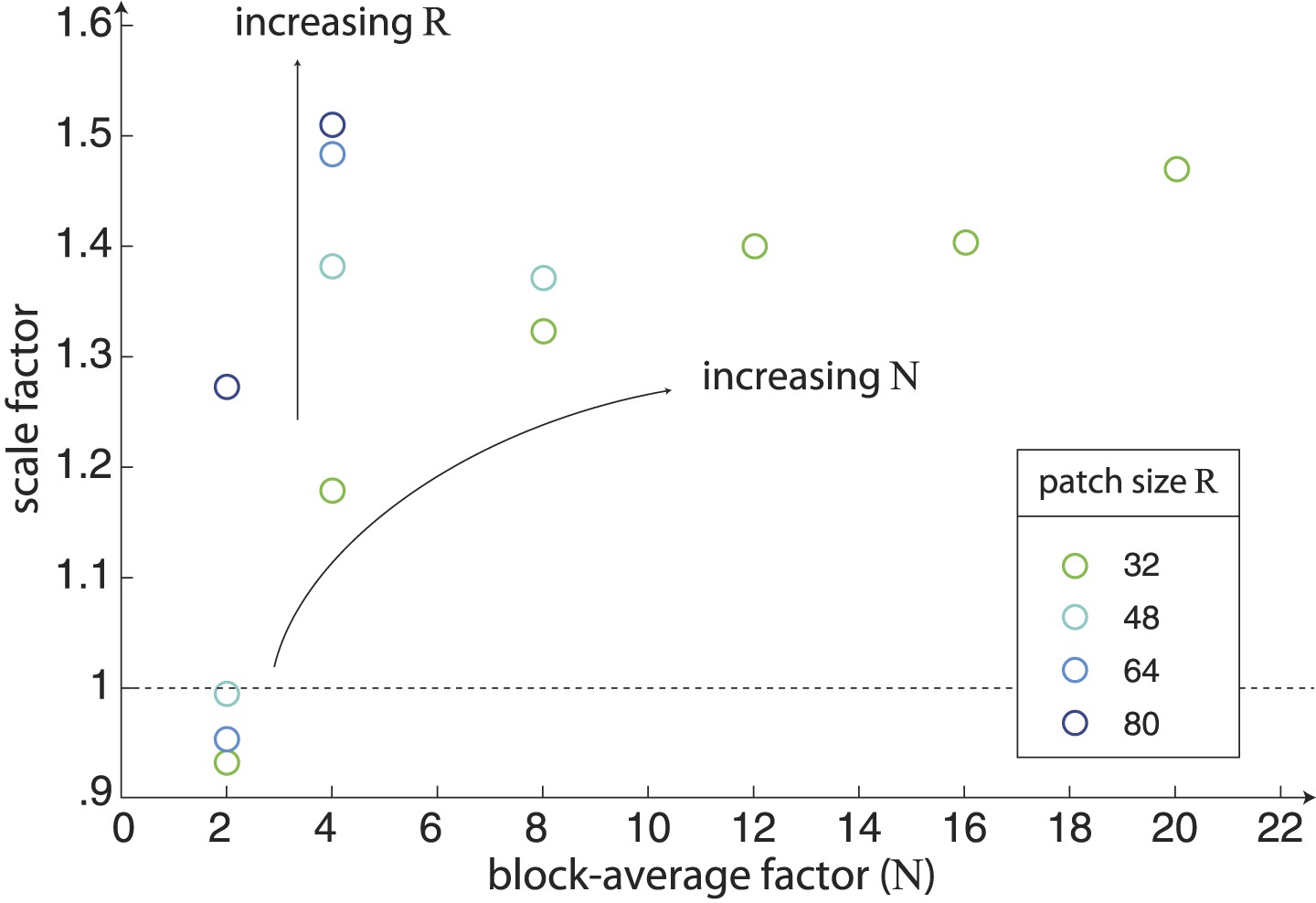
Scaling of natural image analyses.
We scale each image analysis by a single scale factor that minimizes the squared error between the set of nine standard deviations and the set of nine psychophysical sensitivities. The scale factors are shown here as a function of block-average factor N for different choices of the patch size R. We find that the variance of image statistics decreases with increasing values of N, and thus larger values of N require a larger scale factor. Similarly, for a given value of N, the variance of image statistics increases with increasing R, and thus larger values of R require a larger scale factor.
Figure 3—figure supplement 2
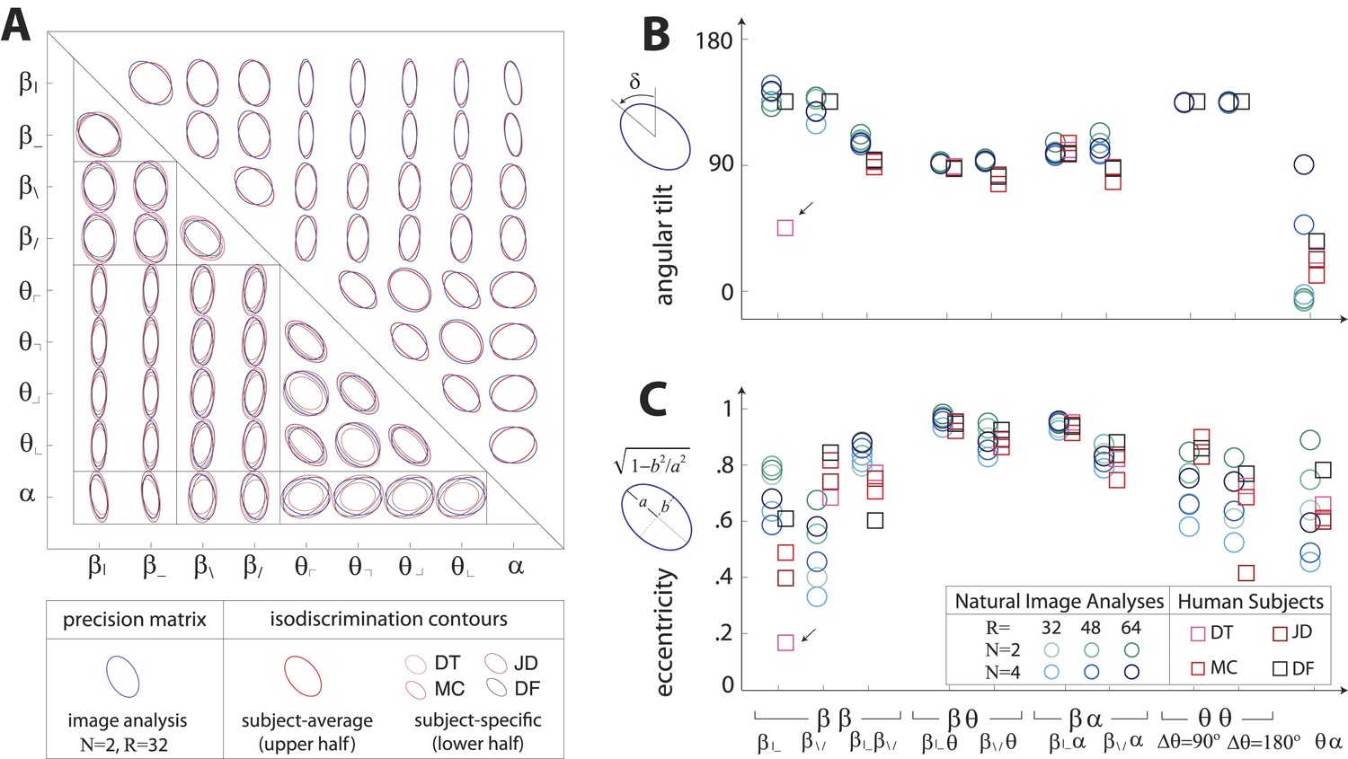
Covariation in natural image statistics predicts human isodiscrimination contours.
(A) For each pair of coordinates, we compare the precision matrix (blue ellipses) extracted from natural scenes (using N =2, R = 32) to human perceptual isodiscrimination contours (red ellipses). Coordinate planes are organized into a grid, with subject-averaged and subject-specific isodiscrimination contours shown respectively above and below the diagonal of the grid. Across all 36 coordinate planes, there is a correspondence in the shape, size, and orientation of precision matrix contours and perceptual isodiscrimination contours. The quality of the match is quantified by computing the angular tilt (B) and eccentricity (C) of image-statistic contours (blue circular markers; shown for variations in the block-average factor (N) and patch size (R) used during image preprocessing) and of perceptual isodiscrimination contours (red square markers; shown for individual subjects). Since contours are highly similar within subsets of coordinate planes (denoted by blocks in A; e.g. the set of planes), contour properties have been averaged within such subsets. Angular tilt and eccentricity are highly consistent between precision matrix contours and perceptual isodiscrimination contours (except for near-circular contours, for which tilt is poorly-defined, as in the case denoted by an arrow).
Figure 3—figure supplement 3
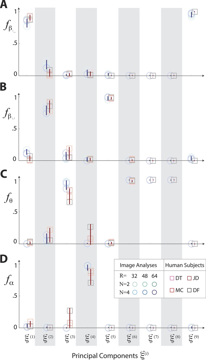
Principal axes of variation in natural images predict principal axes of perceptual sensitivity.
Principal axes of variation in the distribution of natural image statistics are shown in comparison to the principal axes of human sensitivity. Each of the nine principal axes is represented by a vertical gray/white column. Markers (circular = variation in natural image coordinates; square = human perceptual sensitivity) represent the fractional power of the contributions of (A) second-order cardinal (), (B) second-order oblique (), (C) third-order (θ), and (D) fourth-order (α) coordinates to each principal axis; all contributions within each column sum to 1. Principal axes components, and the range of variability observed across image analysis variants or across subjects (see legend), are shown in blue for natural scene statistics and in red for perceptual sensitivities.
Figure 3—figure supplement 4
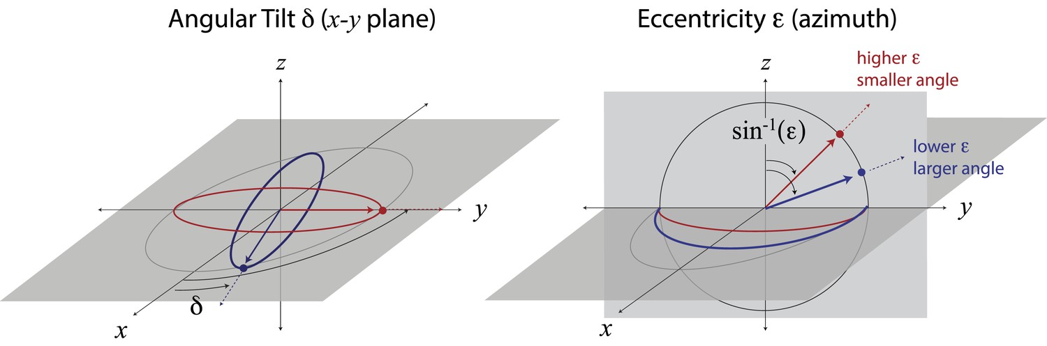
Mapping ellipse shapes to the quarter unit sphere.
We describe an ellipse by the unit vector , where is the eccentricity and δ is the angular tilt. In spherical coordinates, the tilt δ is the polar angle defined in the x−y plane, and the angle is the azimuthal angle measured from the z-direction. In this representation, the unit vector corresponds to a circle, and the unit vectors and correspond, respectively, to the ellipses that have been maximally elongated (i.e., into lines) in the and directions. Points between the equator (in the x−y plane) and the pole correspond to ellipses of intermediate eccentricities.
Figure 3—figure supplement 5
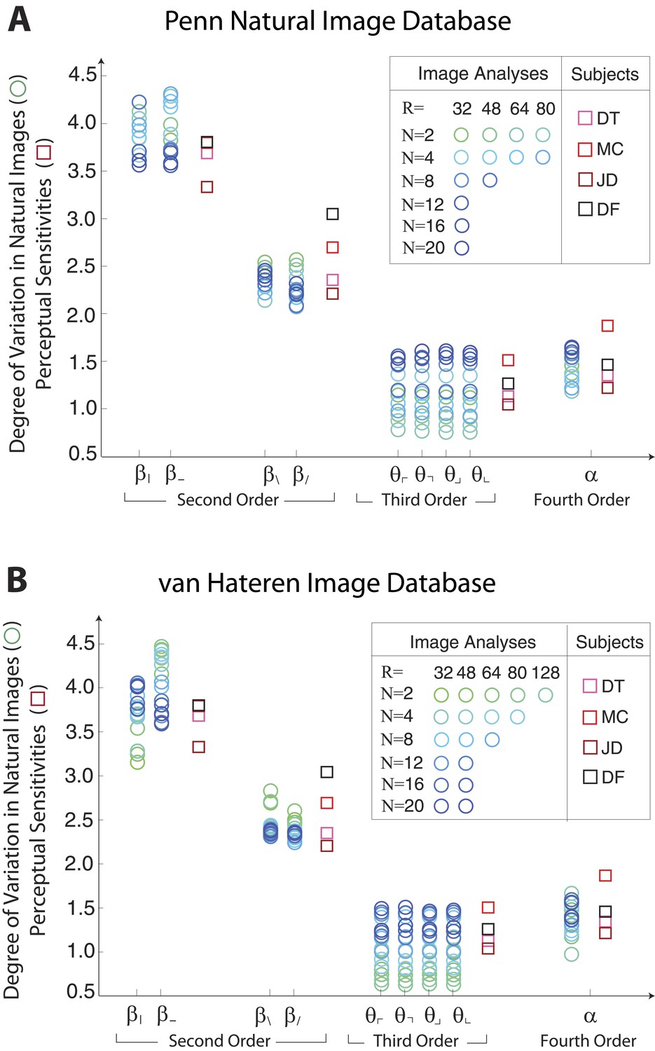
Single coordinate axes: variation in natural images predicts human perceptual sensitivities.
Scaled variation in natural image statistics measured along second- (β), third- (θ), and fourth-order (α) coordinate axes (blue circular markers) are shown in comparison to human perceptual sensitivities measured along the same coordinates (red square markers). Natural image statistics are extracted from the Penn natural image database (A) and the van Hateren image database (B). Ranges of variation and human sensitivities are robustly rank-ordered as . When each image analysis is scaled by a single factor, ranges match sensitivities.
Figure 3—figure supplement 6
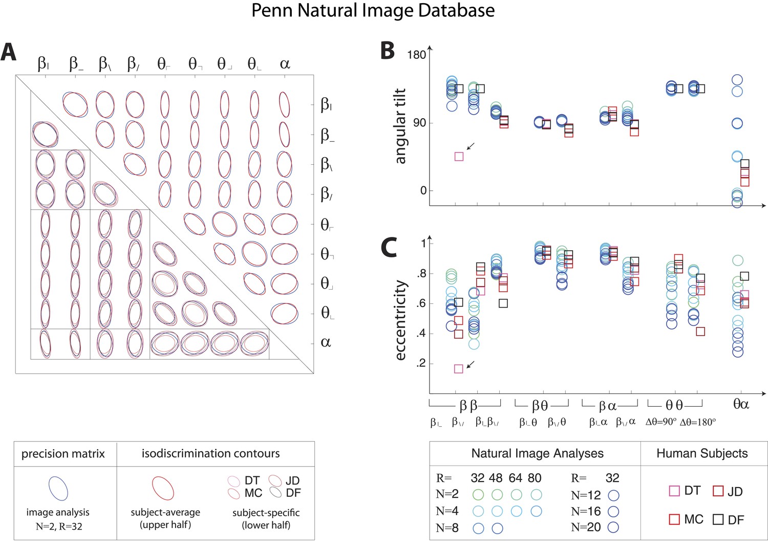
Pairwise coordinate planes in Penn Natural Image Database: covariation in natural images predicts human isodiscrimination contours.
(A) For each pair of coordinates, we compare the precision matrix (blue ellipses) extracted from natural scenes (using N = 2, R = 32) to human perceptual isodiscrimination contours (red ellipses). A precision matrix is represented by the contour lines of its inverse (the covariance matrix M); these are the points (x,y) at which constant. A short distance of the blue contour from the origin thus indicates a large value of M and a small value of the precision matrix. This in turn denotes a direction in which prior knowledge of the image statistic is imprecise. Our prediction is that psychophysical thresholds (red ellipses) should match these contours. Coordinate planes are organized into a grid, with subject-averaged and subject-specific isodiscrimination contours shown respectively above and below the diagonal of the grid. Across all 36 pairwise coordinate planes, there is a correspondence in the shape, size, and orientation of precision matrix contours and perceptual isodiscrimination contours. The quality of the match is quantified by computing the (B) angular tilt and (C) eccentricity of image-statistic contours (circular markers) and of perceptual isodiscrimination contours (square markers). Since contours are highly similar within subsets of pairwise planes (denoted by blocks in A; e.g. the set of planes), contour properties have been averaged within such subsets. Angular tilt and eccentricity are highly consistent between precision matrix contours and perceptual isodiscrimination contours.
Figure 3—figure supplement 7
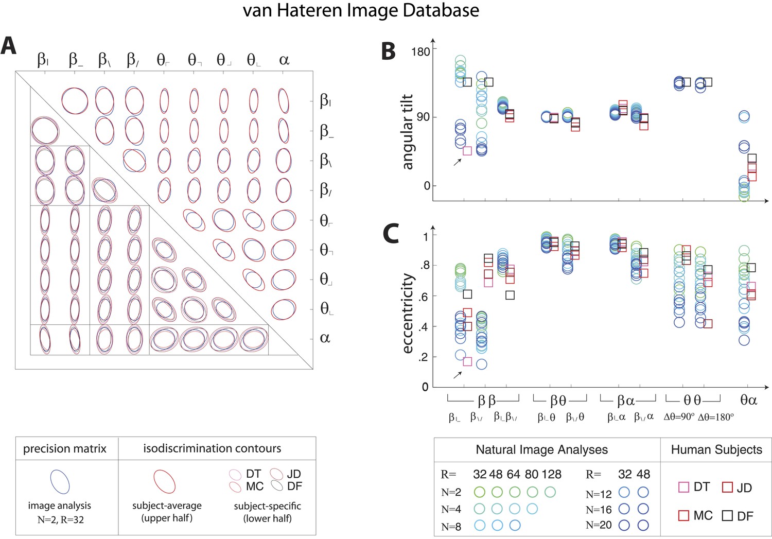
Pairwise coordinate planes in van Hateren Image Database: covariation in natural images predicts human isodiscrimination contours.
(A) For each pair of coordinates, we compare the precision matrix (blue ellipses) extracted from natural scenes (using N = 2, R = 32) to human perceptual isodiscrimination contours (red ellipses). A precision matrix is represented by the contour lines of its inverse (the covariance matrix M); these are the points (x,y) at which constant. A short distance of the blue contour from the origin thus indicates a large value of M and a small value of the precision matrix. This in turn denotes a direction in which prior knowledge of the image statistic is imprecise. Our prediction is that psychophysical thresholds (red ellipses) should match these contours. Coordinate planes are organized into a grid, with subject-averaged and subject-specific isodiscrimination contours shown respectively above and below the diagonal of the grid. Across all 36 pairwise coordinate planes, there is a correspondence in the shape, size, and orientation of precision matrix contours and perceptual isodiscrimination contours. The quality of the match is quantified by computing the (B) angular tilt and (C) eccentricity of image-statistic contours (circular markers) and of perceptual isodiscrimination contours (square markers). Since contours are highly similar within subsets of pairwise planes (denoted by blocks in A; e.g. the set of planes), contour properties have been averaged within such subsets. Angular tilt and eccentricity are highly consistent between precision matrix contours and perceptual isodiscrimination contours. Coordinates extracted from the van Hateren database show larger variability in the and planes than those extracted from the Penn Natural Image Database (Figure 3—figure supplement 6), exhibiting a larger number of low-eccentricity contours for which tilt is poorly defined.
Figure 3—figure supplement 8
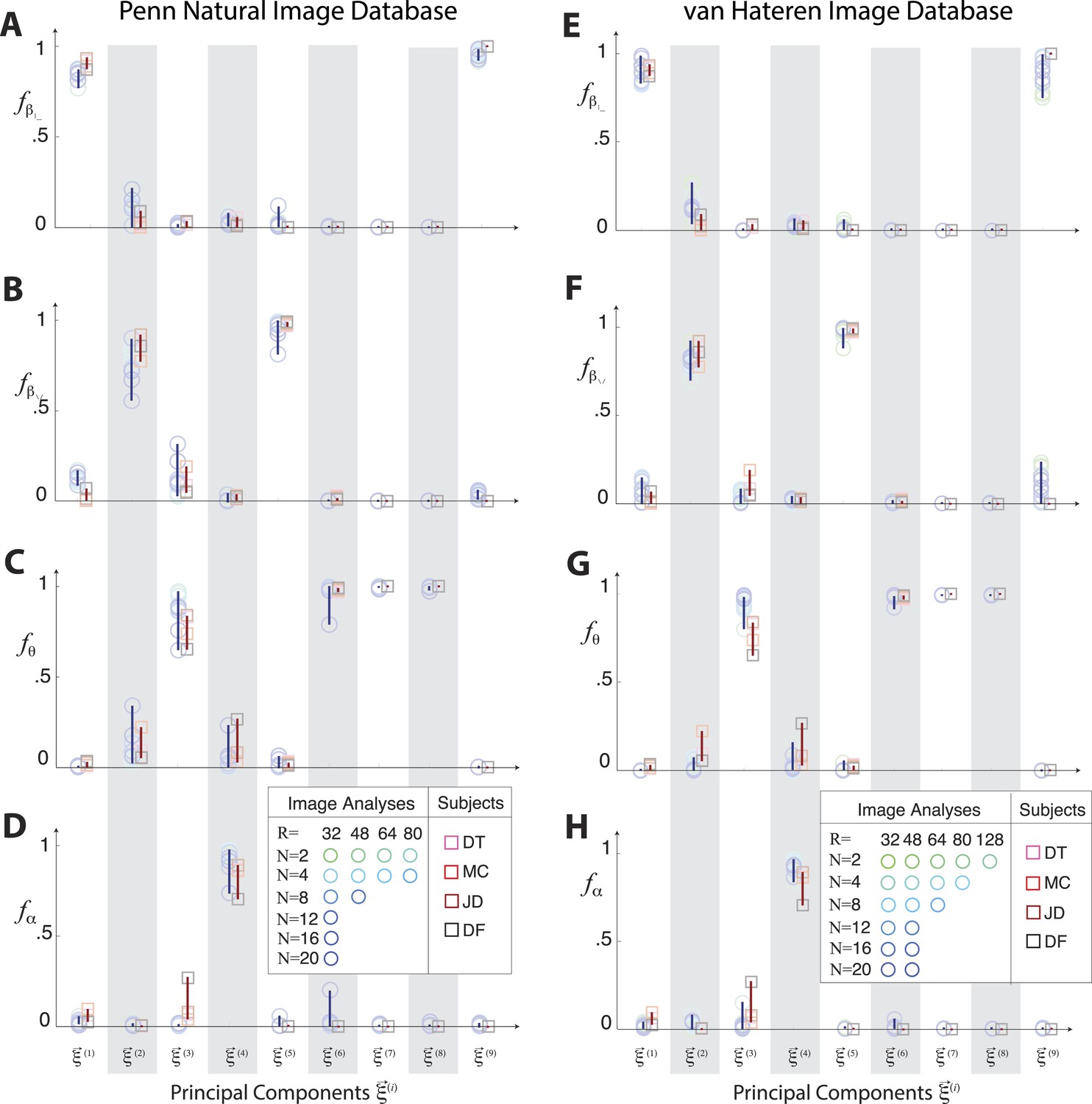
Principal axes of variation across natural images predict principal axes of human perceptual sensitivity in the full coordinate space.
Principal axes of variation in the distribution of natural image statistics are shown in comparison to the principal axes of human sensitivity. Each of the nine principal axes is represented by a vertical gray/white column. Markers (circular = variation in natural image coordinates; square = human perceptual sensitivity) represent the fractional power of the contributions of (A, E) second-order cardinal (), (B, F) second-order oblique (), C, G third-order (θ), and (D, H) fourth-order (α) coordinates to each principal axis; all contributions within each column sum to 1. Principal axes components, and the range of variability observed across image analysis variants or across subjects (see legend), are shown in blue for natural scene statistics and in red for perceptual sensitivities. There is an excellent match between the blue and red components for both the Penn and van Hateren image databases.
Figure 3—figure supplement 9
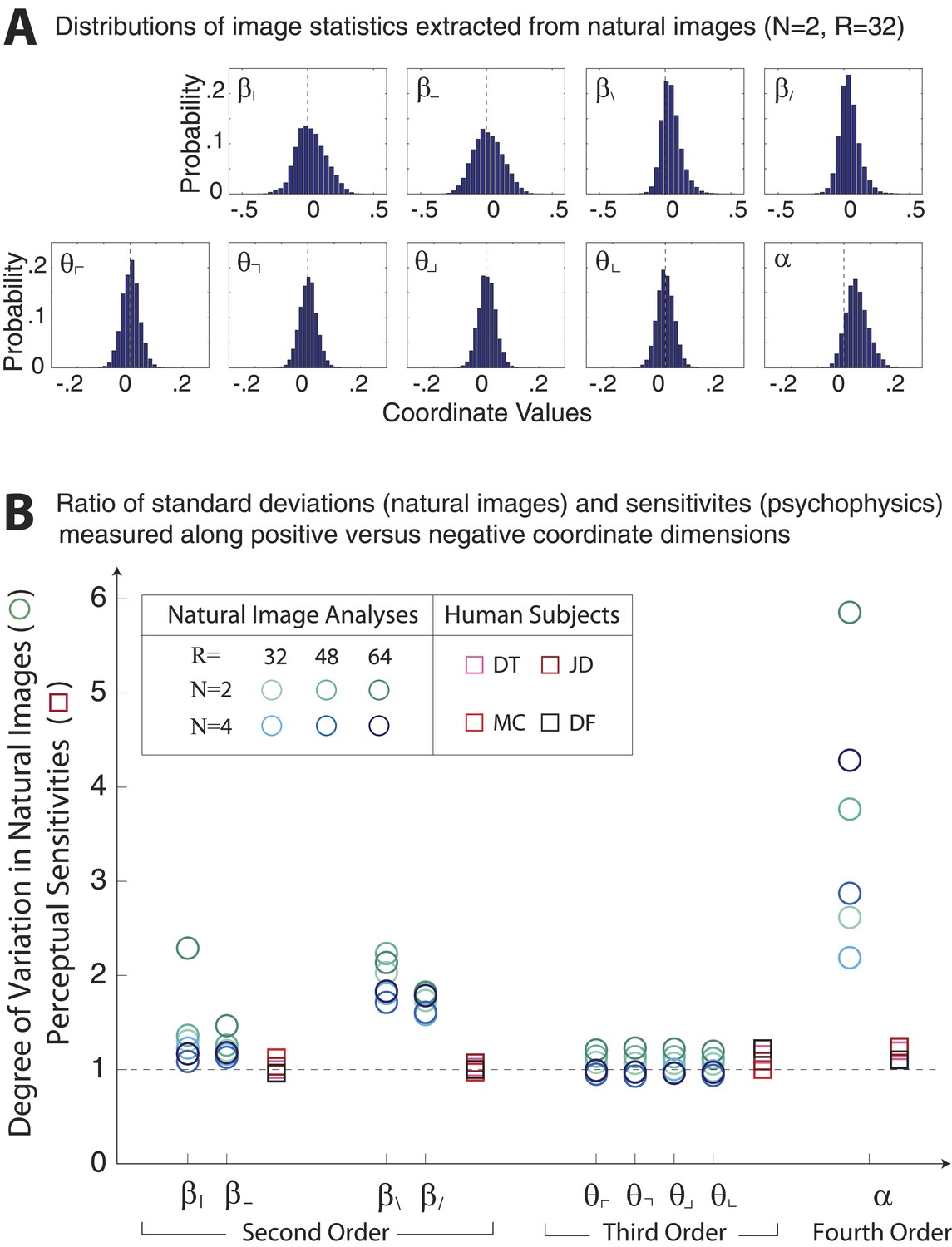
Asymmetries in natural image statistics.
(A) Probability distributions of natural image statistics. Projections of the distribution along second- and fourth-order coordinate axes are asymmetric about the origin, being shifted toward positive values. (B) We compute the ratio of standard deviations measured along positive vs negative coordinate axes (circular markers) to the ratio of human sensitivities measured along positive vs negative coordinate axes (square markers). Natural images show larger asymmetries in second- and fourth-order coordinate values than is observed in human sensitivities. This is particularly notable for the α coordinate, which shows a 2–6 fold asymmetry in natural images variation but at most a 1.2-fold asymmetry in human sensitivity.
Figure 4 with 4 supplements
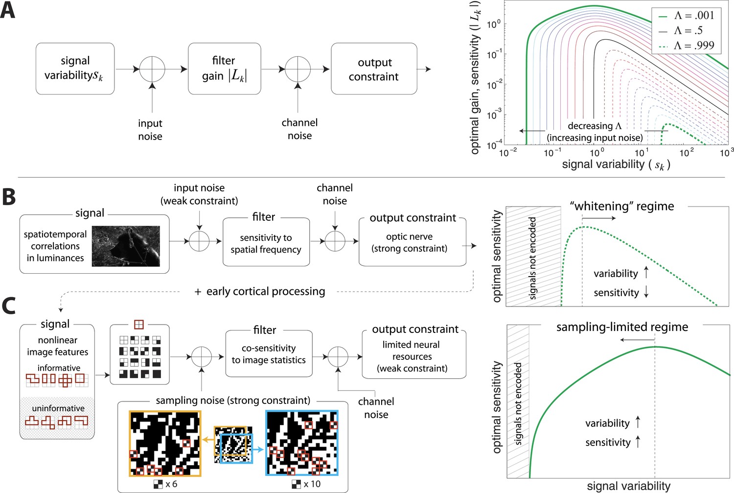
Regimes of efficient coding.
(A) To analyze different regimes of efficient coding, we consider a set of channels, where the channel carries an input signal with variability . Gaussian noise is added to the input. The result is passed through a linear filter with gain , and then Gaussian noise is added to the filter output. We impose a constraint on the total power output of all channels, that is, a constraint on its total resources. With these assumptions, the set of gains that maximizes the transmitted information can be determined (see ‘Materials and methods’, Two regimes of efficient coding, and (van Hateren, 1992a; Doi and Lewicki, 2011; Doi and Lewicki, 2014)). This set of gains depends on the relative strengths of input and output noise and on the severity of the power constraint, quantified here by the dimensionless parameter (right-hand panel). As decreases from 1 to 0, the system moves from a regime in which output noise is limiting to one in which input noise is limiting. (B) The efficient coding model applied to the sensory periphery. Raw luminances from natural images are corrupted with noise (e.g. shot noise resulting from photon incidence) and passed through a linear filter. The resulting signal is carried by the optic nerve, which imposes a strong constraint on output capacity. In the bandwidth limited case where output noise dominates over input noise (e.g., under high light conditions when photon noise is not limiting), the optimal gain decreases as signal variability increases. Since channel input and channel gain vary reciprocally, channel outputs are approximately equalized, resulting in a ‘whitening’, or decorrelation. (C) The efficient coding model applied to cortical processing. Informative image features resulting from early cortical processing, caricatured by our preprocessing pipeline as applied to the retinal output, are sampled from a spatial region of the image. This sampling acts as a kind of input noise, because it only provides limited count-based estimates for the true statistical properties of the image source. When this input noise is limiting, the optimal gain increases as signal variability increases. Rather than whiten, the output signals preserve the correlational structure of the input. Note that in both regimes (B) and (C), there is a range of signals that are not encoded at all. These are the signals that are not sufficiently informative to warrant an allocation of resources.
Figure 4—figure supplement 1
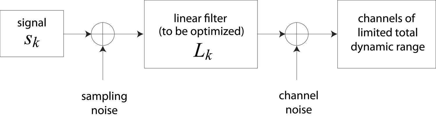
Schematic representation of channel optimization problem.
We consider a set of channels, each of which is dedicated to processing an independent signal . Sampling noise (taken here to be unity) is added to the signal , which is then passed through a linear filter with gain . Channel noise (taken here to be unity) is added to the output of . The total dynamic range of all channels is constrained.
Figure 4—figure supplement 2
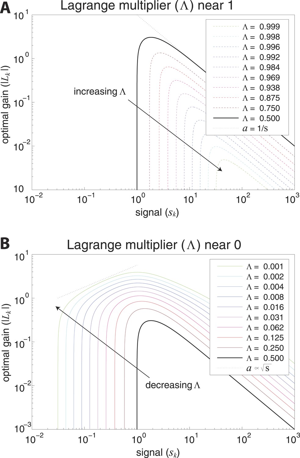
Optimal coding regimes.
Optimal gain is shown as a function of signal strength for different choices of the output constraint . For signals below a critical strength , the optimal gain is zero, and signals are not encoded. The limit from below defines the transmission-limited regime, while the limit from above defines the sampling-limited regime. (A) Transmission-limited regime. For signal strengths much larger than the critical value, the main constraint is output power, and the optimal gain is inversely proportional to the signal strength (as indicated by the dotted line with negative slope). As , there is an increasingly sharp transition between signals that are not encoded, and signals that are encoded in inverse proportion to their size (‘whitened’). (B) Sampling-limited regime. As , there is a broadening of the transition between signals that are not encoded, and signals that are whitened. This broadening results in a regime in which sampling-noise is the dominant constraint, and the optimal gain increases with signal strength (as indicated by the dotted line with positive slope).
Figure 4—figure supplement 3
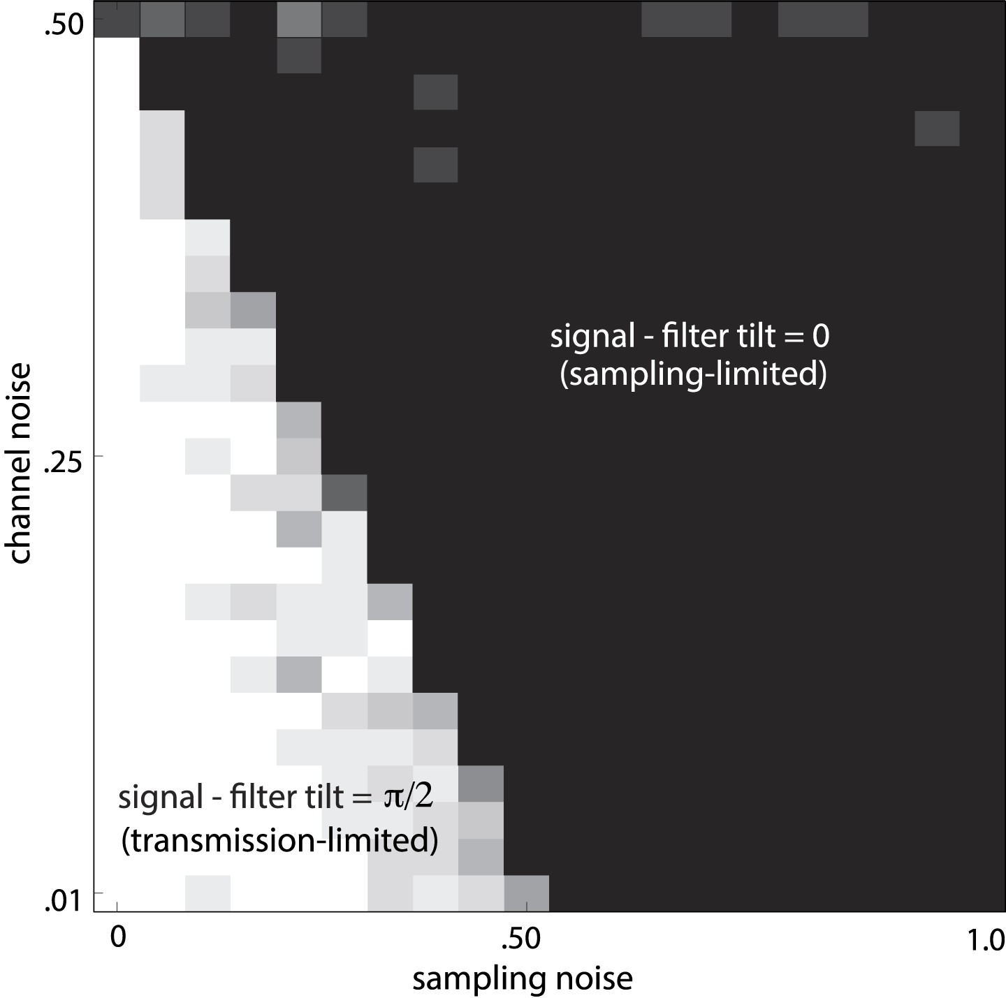
Noise-dependent transition between efficient coding regimes.
Total noise is the sum of sampling noise (x-axis) and channel noise (y-axis). In the case considered here (d = 2), channel noise cannot exceed 0.5, but sampling noise can. For total noise below 0.5, the optimal filter L is antialigned with the signal, and the optimal strategy is decorrelation via whitening (white region, transmission-limited regime). For total noise above 0.5, the optimal filter is aligned with the signal (black region, sampling-limited regime), consistent with our findings that perceptual sensitivity is tuned to the direction and degree of variation in natural image statistics.
Figure 4—figure supplement 4
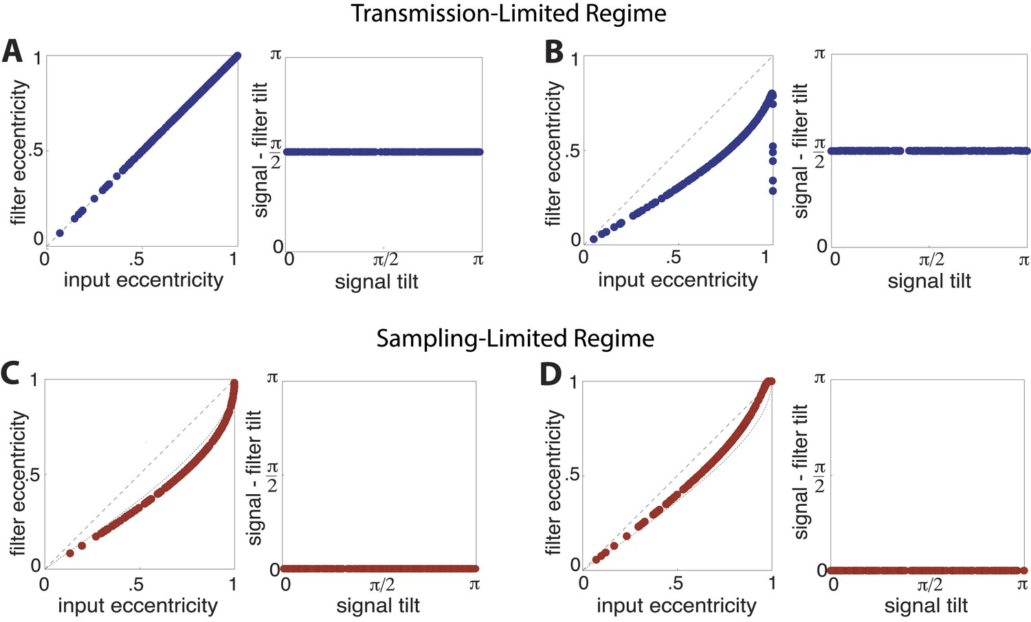
Optimal filter shape and orientation.
Tilt and eccentricity of the optimal linear filter for random choices of the input signal s. As the magnitudes of sampling and channel noises vary, there emerge two regimes of efficient coding: a transmission-limited regime (A–B) and a sampling-limited regime (C–D). In the transmission-limited regime, the maximum filter eigendirection is aligned with the minimum signal eigendirection (and hence there is a difference in tilt of ). In contrast, in the sampling-limited regime, the maximum filter eigendirection is aligned with the maximum signal eigendirection. Note that a direct comparison of eccentricities between these two regimes can be misleading, due to a reversal of the maximal eigendirections. (A) Sampling noise , channel noise . The optimal strategy is decorrelation via whitening using a filter aligned perpendicularly to the input signal (right panel) with an eccentricity that matches that of the input signal (dashed line, left panel). (B) Sampling noise , channel noise . At very low total noise, even with zero channel noise, the optimal strategy is still decorrelation (right panel) using a filter whose eccentricity is less than the eccentricity of the input signal. (C) Sampling noise , channel noise (the low input SNR regime identified in (van Hateren, 1992a)). The tilt of the optimal filter is aligned to the tilt of the signal (right panel), and the filter eccentricity is approaching the prediction of the square-root gain relation (curved dotted line, left panel) with decreasing SNR. (D) Sampling noise , channel noise (dominating sampling noise). For increasing sampling noise strength, the filter eccentricities match the signal eccentricities (dashed line, left panel).
Tables
Table 1
Permutation tests for null model 1a: shuffled coordinate labels
| Measures of overlap | Image analysis | Observed overlap | Shuffled overlap Values | Significance | ||||
|---|---|---|---|---|---|---|---|---|
| Mean | std | min | max | |||||
| Range/Sensitivity | N = 2 | R = 32 | 0.999 | 0.859 | 0.9 × 10⁻¹ | 0.704 | 0.983 | <0.04 |
| R = 48 | 0.993 | 0.832 | 1.1 × 10⁻¹ | 0.651 | 0.978 | <0.04 | ||
| R = 64 | 0.987 | 0.809 | 1.1 × 10⁻¹ | 0.614 | 0.974 | <0.04 | ||
| N = 4 | R = 32 | 0.998 | 0.825 | 1.1 × 10⁻¹ | 0.638 | 0.969 | <0.04 | |
| R = 48 | 0.994 | 0.812 | 1.1 × 10⁻¹ | 0.646 | 0.990 | <0.04 | ||
| R = 64 | 0.991 | 0.794 | 1.1 × 10⁻¹ | 0.617 | 0.985 | <0.04 | ||
| Inverse Range/Threshold | N = 2 | R = 32 | 0.971 | 0.709 | 1.5 × 10⁻¹ | 0.508 | 0.924 | <0.04 |
| R = 48 | 0.969 | 0.692 | 1.6 × 10⁻¹ | 0.469 | 0.924 | <0.04 | ||
| R = 64 | 0.953 | 0.685 | 1.7 × 10⁻¹ | 0.450 | 0.913 | <0.04 | ||
| N = 4 | R = 32 | 0.967 | 0.679 | 1.7 × 10⁻¹ | 0.447 | 0.908 | <0.04 | |
| R = 48 | 0.975 | 0.632 | 1.5 × 10⁻¹ | 0.400 | 0.880 | <0.04 | ||
| R = 64 | 0.977 | 0.648 | 1.6 × 10⁻¹ | 0.411 | 0.894 | <0.04 | ||
| Fractional Principal Components | N = 2 | R = 32 | 0.994 | 0.382 | 1.5 × 10⁻¹ | 0.160 | 0.657 | <0.04 |
| R = 48 | 0.995 | 0.485 | 1.2 × 10⁻¹ | 0.287 | 0.727 | <0.04 | ||
| R = 64 | 0.991 | 0.487 | 0.7 × 10⁻¹ | 0.372 | 0.632 | <0.04 | ||
| N = 4 | R = 32 | 0.995 | 0.459 | 1.4 × 10⁻¹ | 0.238 | 0.732 | <0.04 | |
| R = 48 | 0.996 | 0.444 | 1.0 × 10⁻¹ | 0.277 | 0.601 | <0.04 | ||
| R = 64 | 0.996 | 0.450 | 1.1 × 10⁻¹ | 0.279 | 0.614 | <0.04 | ||
| Full Principal Components | N = 2 | R = 32 | 0.917 | 0.316 | 1.3 × 10⁻¹ | 0.123 | 0.578 | <0.04 |
| R = 48 | 0.828 | 0.401 | 1.0 × 10⁻¹ | 0.228 | 0.611 | <0.04 | ||
| R = 64 | 0.911 | 0.363 | 0.7 × 10⁻¹ | 0.282 | 0.532 | <0.04 | ||
| N = 4 | R = 32 | 0.882 | 0.376 | 1.2 × 10⁻¹ | 0.180 | 0.618 | <0.04 | |
| R = 48 | 0.917 | 0.362 | 1.0 × 10⁻¹ | 0.201 | 0.520 | <0.04 | ||
| R = 64 | 0.919 | 0.357 | 1.0 × 10⁻¹ | 0.196 | 0.522 | <0.04 | ||
-
We separately permute the sets of coordinate labels . We apply these permutations to the psychophysical data, therein examining all 23 non-identity permutations of the four labels. This shuffling significantly decreases the overlap between image analyses and psychophysical data. Results are significant across all six analyses considered in Figures 1 and 3 (N = 2, 4 and R = 32, 48, 64). p-values, estimated as the fraction of permutations for which the shuffled overlap exceeds the true overlap, are less than 0.04 (the minimum value given 23 permutations) for each image analysis.
Table 2
Permutation Tests for null model 1b: shuffled coordinate labels
| Measures of overlap | Image analysis | Observed overlap | Shuffled overlap Values | Significance | ||||
|---|---|---|---|---|---|---|---|---|
| Mean | std | min | max | |||||
| Range/Sensitivity | N = 2 | R = 32 | 0.999 | 0.806 | 6.8 × 10⁻² | 0.659 | 0.999 | 0.0003 |
| R = 48 | 0.993 | 0.775 | 7.7 × 10⁻² | 0.610 | 0.993 | <0.0001 | ||
| R = 64 | 0.987 | 0.762 | 8.0 × 10⁻² | 0.579 | 0.987 | <0.0001 | ||
| N = 4 | R = 32 | 0.998 | 0.828 | 6.0 × 10⁻² | 0.707 | 0.998 | <0.0001 | |
| R = 48 | 0.994 | 0.798 | 7.1 × 10⁻² | 0.660 | 0.994 | 0.0002 | ||
| R = 64 | 0.991 | 0.780 | 7.6 × 10⁻² | 0.630 | 0.991 | <0.0001 | ||
| Inverse Range/Threshold | N = 2 | R = 32 | 0.971 | 0.693 | 8.1 × 10⁻² | 0.499 | 0.972 | 0.0002 |
| R = 48 | 0.969 | 0.682 | 8.4 × 10⁻² | 0.476 | 0.969 | 0.0003 | ||
| R = 64 | 0.953 | 0.671 | 8.5 × 10⁻² | 0.446 | 0.954 | 0.0002 | ||
| N = 4 | R = 32 | 0.967 | 0.696 | 7.6 × 10⁻² | 0.521 | 0.964 | <0.0001 | |
| R = 48 | 0.975 | 0.692 | 8.0 × 10⁻² | 0.509 | 0.976 | 0.0002 | ||
| R = 64 | 0.977 | 0.689 | 8.2 × 10⁻² | 0.493 | 0.978 | 0.0003 | ||
| Fractional Principal Components | N = 2 | R = 32 | 0.994 | 0.592 | 1.2 × 10⁻¹ | 0.271 | 0.995 | 0.0003 |
| R = 48 | 0.995 | 0.604 | 1.3 × 10⁻¹ | 0.281 | 0.995 | 0.0004 | ||
| R = 64 | 0.991 | 0.591 | 1.2 × 10⁻¹ | 0.278 | 0.991 | 0.0003 | ||
| N = 4 | R = 32 | 0.995 | 0.590 | 1.2 × 10⁻¹ | 0.218 | 0.995 | 0.0001 | |
| R = 48 | 0.996 | 0.577 | 1.2 × 10⁻¹ | 0.251 | 0.996 | 0.0002 | ||
| R = 64 | 0.996 | 0.581 | 1.2 × 10⁻¹ | 0.266 | 0.996 | 0.0004 | ||
| Full Principal Components | N = 2 | R = 32 | 0.917 | 0.391 | 1.2 × 10⁻¹ | 0.100 | 0.927 | 0.0002 |
| R = 48 | 0.828 | 0.391 | 1.2 × 10⁻¹ | 0.086 | 0.856 | 0.0008 | ||
| R = 64 | 0.911 | 0.396 | 1.2 × 10⁻¹ | 0.120 | 0.953 | 0.0003 | ||
| N = 4 | R = 32 | 0.882 | 0.381 | 1.2 × 10⁻¹ | 0.066 | 0.989 | 0.0003 | |
| R = 48 | 0.917 | 0.380 | 1.2 × 10⁻¹ | 0.090 | 0.902 | <0.0001 | ||
| R = 64 | 0.919 | 0.387 | 1.2 × 10⁻¹ | 0.095 | 0.937 | 0.0004 | ||
-
We separately permute all nine coordinate labels . This shuffling, applied to the psychophysical data, significantly decreases the overlap between image analyses and psychophysical data. Results are significant across all six analyses considered in Figures 1 and 3 (N = 2, 4 and R = 32, 48, 64). p-values, estimated as the fraction of permutations for which the shuffled overlap exceeds the true overlap, are less than 0.0005 for all image analyses.
Table 3
Permutation tests for null model 2: shuffled patch labels
| Comparisons | Image analysis | Observed overlap | Shuffled overlap Values | Significance | ||||
|---|---|---|---|---|---|---|---|---|
| Mean | std | min | max | |||||
| Inverse Range/Threshold | N = 2 | R = 32 | 0.971 | 0.924 | 0.70 × 10⁻³ | 0.921 | 0.926 | <0.0001 |
| R = 48 | 0.969 | 0.921 | 1.1 × 10⁻³ | 0.917 | 0.925 | <0.0001 | ||
| R = 64 | 0.953 | 0.912 | 1.3 × 10⁻³ | 0.908 | 0.917 | <0.0001 | ||
| N = 4 | R = 32 | 0.967 | 0.919 | 1.7 × 10⁻³ | 0.914 | 0.926 | <0.0001 | |
| R = 48 | 0.975 | 0.922 | 1.9 × 10⁻³ | 0.916 | 0.930 | <0.0001 | ||
| R = 64 | 0.977 | 0.924 | 2.8 × 10⁻³ | 0.916 | 0.935 | <0.0001 | ||
| Fractional Principal Components | N = 2 | R = 32 | 0.994 | 0.806 | 9.1 × 10⁻⁶ | 0.806 | 0.806 | <0.0001 |
| R = 48 | 0.995 | 0.806 | 8.3 × 10⁻⁶ | 0.806 | 0.806 | <0.0001 | ||
| R = 64 | 0.991 | 0.806 | 3.7 × 10⁻⁶ | 0.806 | 0.806 | <0.0001 | ||
| N = 4 | R = 32 | 0.995 | 0.807 | 2.5 × 10⁻⁴ | 0.806 | 0.809 | <0.0001 | |
| R = 48 | 0.996 | 0.807 | 4.1 × 10⁻⁴ | 0.806 | 0.810 | <0.0001 | ||
| R = 64 | 0.996 | 0.807 | 3.5 × 10⁻⁴ | 0.806 | 0.810 | <0.0001 | ||
| Full Principal Components | N = 2 | R = 32 | 0.917 | 0.448 | 5.8 × 10⁻² | 0.406 | 0.596 | <0.0001 |
| R = 48 | 0.828 | 0.502 | 5.9 × 10⁻² | 0.408 | 0.675 | <0.0001 | ||
| R = 64 | 0.911 | 0.458 | 4.8 × 10⁻² | 0.407 | 0.591 | <0.0001 | ||
| N = 4 | R = 32 | 0.881 | 0.489 | 4.9 × 10⁻² | 0.409 | 0.638 | <0.0001 | |
| R = 48 | 0.917 | 0.454 | 3.0 × 10⁻² | 0.408 | 0.637 | <0.0001 | ||
| R = 64 | 0.919 | 0.492 | 4.2 × 10⁻² | 0.411 | 0.648 | <0.0001 | ||
-
Within each image analyses, we separately permute image patch labels along individual coordinate axes. This shuffling does not alter the range of variation observed along individual coordinates; as a result, this test only applies to , and . We find that this shuffling significantly decreases the overlap between image analyses and psychophysical data. Results are significant across all six analyses considered in Figures 1 and 3 (N = 2, 4 and R = 32, 48, 64). p-values, estimated as the fraction of permutations for which the shuffled overlap exceeds the true overlap, are less than 0.0001 for each image analysis.
Download links
A two-part list of links to download the article, or parts of the article, in various formats.
Downloads (link to download the article as PDF)
Open citations (links to open the citations from this article in various online reference manager services)
Cite this article (links to download the citations from this article in formats compatible with various reference manager tools)
Variance predicts salience in central sensory processing
eLife 3:e03722.
https://doi.org/10.7554/eLife.03722


