3D imaging of Sox2 enhancer clusters in embryonic stem cells
- Howard Hughes Medical Institute, Janelia Research Campus, United States
- University of California, Berkeley, United States
Figures
Figure 1 with 1 supplement
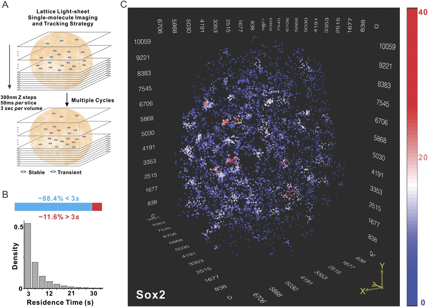
Localization of Sox2 stable binding sites in 3D by lattice light-sheet, single-molecule imaging.
(A) Whole-nucleus single molecule imaging was performed by lattice light-sheet microscopy with 300 nm z steps and 50 ms per frame. HaloTag-Sox2 molecules were labeled by membrane permeable JF549 dye. The imaging scheme was cycled every 3 s for ∼500 times. The 3D positions of single molecule localization events were tracked (for more details, see ‘Materials and methods’). Any Sox2 molecules that dwelled at a position for more than 3 s were counted as stable bound events. See Videos 1 and 2 for the exemplary raw data. (B) Upper: out of total localized and tracked events, only ∼11.6 ± 3.2% had residence times longer than 3 s. ∼88.4 ± 6.5% Sox2 molecules appeared in single frames (n = 9 cells). Lower: residence time histogram of stable bound Sox2 molecules. The average residence time detected by this imaging set-up is ∼6.92 ± 0.51 s (n = 9 cells). (C) 3D density map of stable Sox2 binding sites in single ES cell nucleus. For fair comparisons between experimental conditions, we only considered 7000 stable binding sites for each cell. The color map reflects the number of local neighbors that was calculated by using a canopy radius of 400 nm. The unit of the x, y, z axes is nm. See Video 3 for the full 3D rotation movie.
Figure 1—figure supplement 1
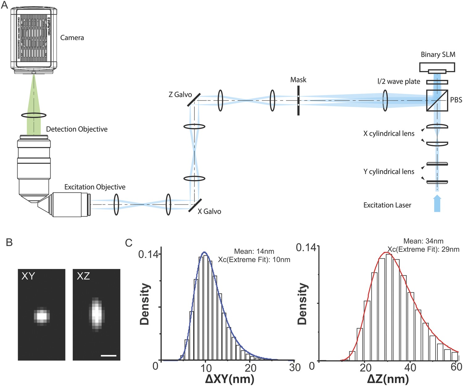
Optics layout, PSF, and localization uncertainty estimation.
(A) Schematic of the light path used for the optical lattice microscope. A collimated circular laser beam is passed through two pairs of cylindrical lenses to illuminate a thin stripe across the width of a ferroelectric spatial light modulator (SLM, Forth Dimension Displays, SXGA-3DM). The remainder of the excitation optical path serves to create a demagnified image of the SLM (81.6 nm pixels) at the focal plane of the excitation objective. First, a lens is used in a 2F configuration to create a diffraction pattern at its front focal plane that is the Fourier transform of the electric field reflected from the SLM. A custom opaque mask with transmissive annuli (Photo-Sciences Inc.) is placed at this plane, and a specific annulus is chosen to remove the unwanted diffraction orders and enforce a limit on the minimum field of view. The electric field transmitted through the mask is then imaged in series onto each of a pair of galvanometers (Cambridge Technology, 6215H) and the rear pupil plane of the excitation objective. The galvanometers serve to translate the light sheet through the specimen in x and z. Finally, the field is reverse transformed by the excitation objective to create the desired lattice light sheet at its front focal plane. The fluorescence generated within the specimen is collected by a detection objective (Nikon, CFI Apo LWD 25XW, 1.1 NA, 2 mm WD) whose focal plane is co-incident with the light sheet. Its high NA is essential to maximize the xy resolution and to optimize the light collection for single molecule detection. The excitation objective (Special Optics, 0.65 NA, 3.74 mm WD) was custom designed to fill the remaining available solid angle above the cover slip. A tube lens images the fluorescence from the illuminated slice within the specimen onto a sCMOS camera (Hamamatsu Orca Flash 4.0 v2) capable of frame rates down to 1 ms. A 3D image is produced from a stack of such 2D slices, either by moving the light sheet and detection objective together through the specimen (the former with the z galvo, the latter with a piezoelectric stage [Physik Instrumente, P-621.1CD]) or, far more commonly, by translating the specimen with a second piezo stage through the stationary light sheet along an axis s in the plane of the specimen cover slip. The specimen holder and specimen piezo are mounted on a trio of closed loop micropositioning stages (Physik Instrumente M-663 for horizontal motion in the cover slip plane, M-122.2DD for vertical travel). (B) The XY and XZ point spread function profile of a fluorescent bead (Emission: ∼590 nm; Voxel size, 100 nm in each direction, the radius of the bead is 50 nm). Scale bar, 500 nm. (C) 3D single-molecule localization was performed using 3D Gaussian model (Equation 1) by FISH-QUANT (Mueller et al., 2013). x, y, z localization uncertainty for each 3D localization event was calculated by using the published estimator, Equation 2. The localization histogram was fitted by Extreme Fit by Matlab. The mean and center values were labeled in each plot.
Figure 2 with 2 supplements
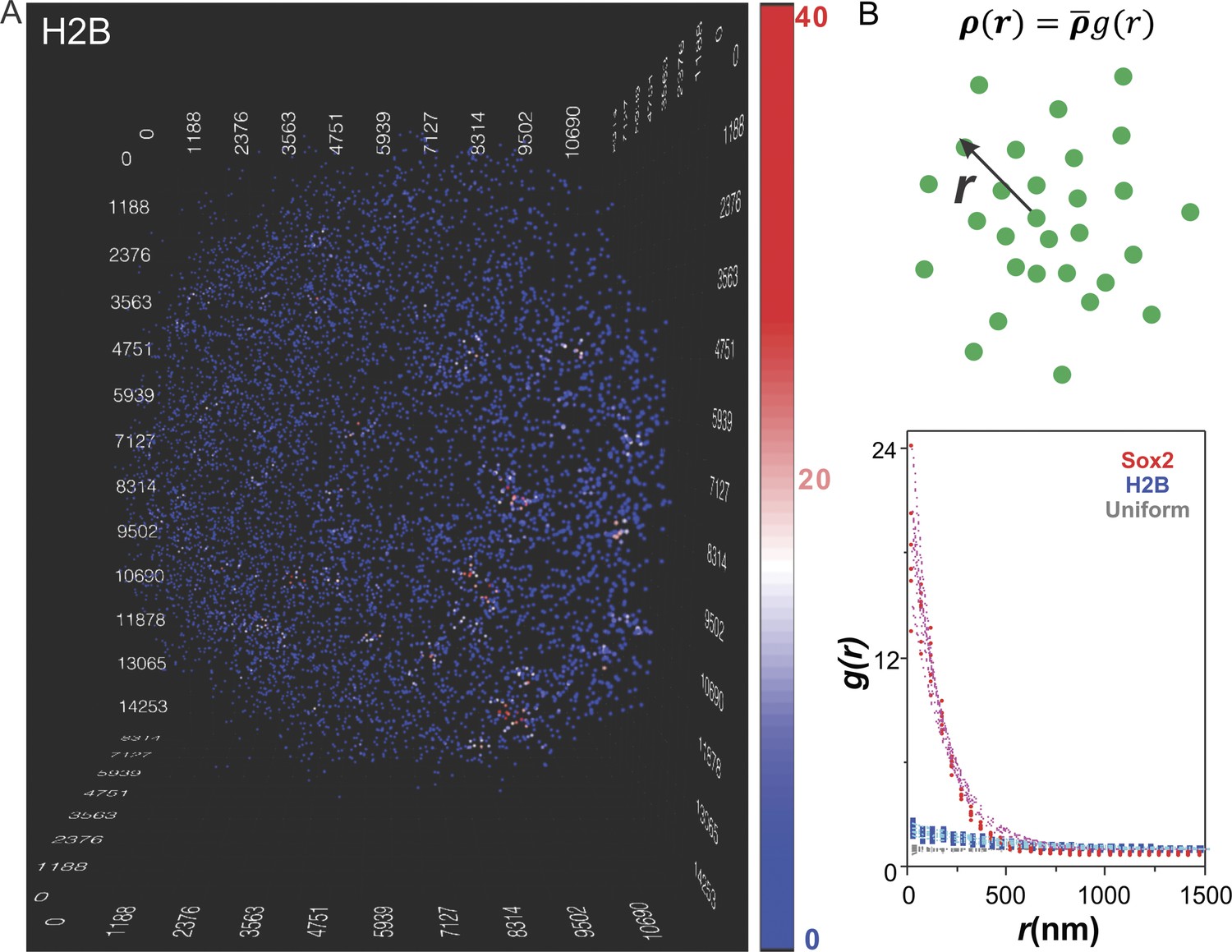
Clustering of Sox2 bound enhancers in the nucleus.
(A) 3D density map of H2B distribution (n = 7000) in single ES cell nucleus. The imaging condition and analysis parameter set-ups were the same as HaloTag-Sox2 in Figure 1. The color map reflects the number of local neighbors that was calculated by using a radius of 400 nm. The unit of the x, y, z axes is nm. See Video 4 for the full 3D rotation movie. (B) Upper: The pair correlation function g(r) measures the relative density of enhancer sites in a volume element at a separation r from single enhancer sites, given that the average density of enhancer sites in the whole volume is . See Equations 3–7 for calculation details. Lower: Pair correlation function of Sox2 stable binding sites (red dots, n = 6), H2B (blue squares, n = 6), and simulated uniformly distributed particles (gray diamond, n = 5, Video 5) fitted with the fluctuation model (dotted lines) (See Equations 10–13). The obtained fluctuation amplitude and range for each curve are in Supplementary file 1.
Figure 2—figure supplement 1
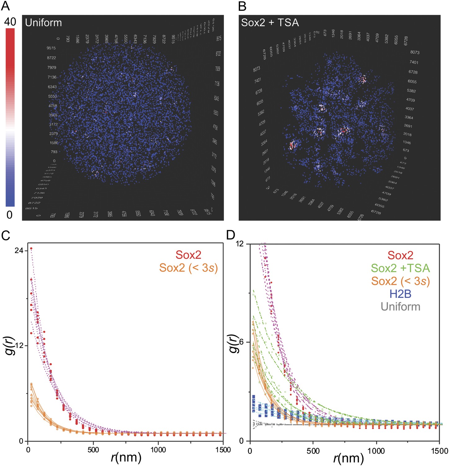
Quantification of clustering by pair correlation function.
(A) 3D density map of simulated uniform sites (n = 7000) in single ES cell nucleus. The color map reflects the number of local neighbors that was calculated by using a canopy radius of 400 nm. The unit of the x, y, z axes is nm. See Video 5 for the full 3D rotation movie. (B) 3D density map of Sox2 stable binding sites (n = 7000) in single TSA treated ES cell nucleus. The color map reflects the number of local neighbors that was calculated by using a canopy radius of 400 nm. The unit of the x, y, z axes is nm. (C) Pair correlation function of Sox2 binding sites that have residence times less than 3 s (yellow, n = 6) fitted with the fluctuation model (dotted lines) (See Equations 10–13). See Video 6 for the full 3D rotation movie. (D) The room-in view of pair correlation function and fluctuation model fitting of the indicated conditions. The obtained fluctuation amplitude and range for each curve are in Supplementary file 1.
Figure 2—figure supplement 2
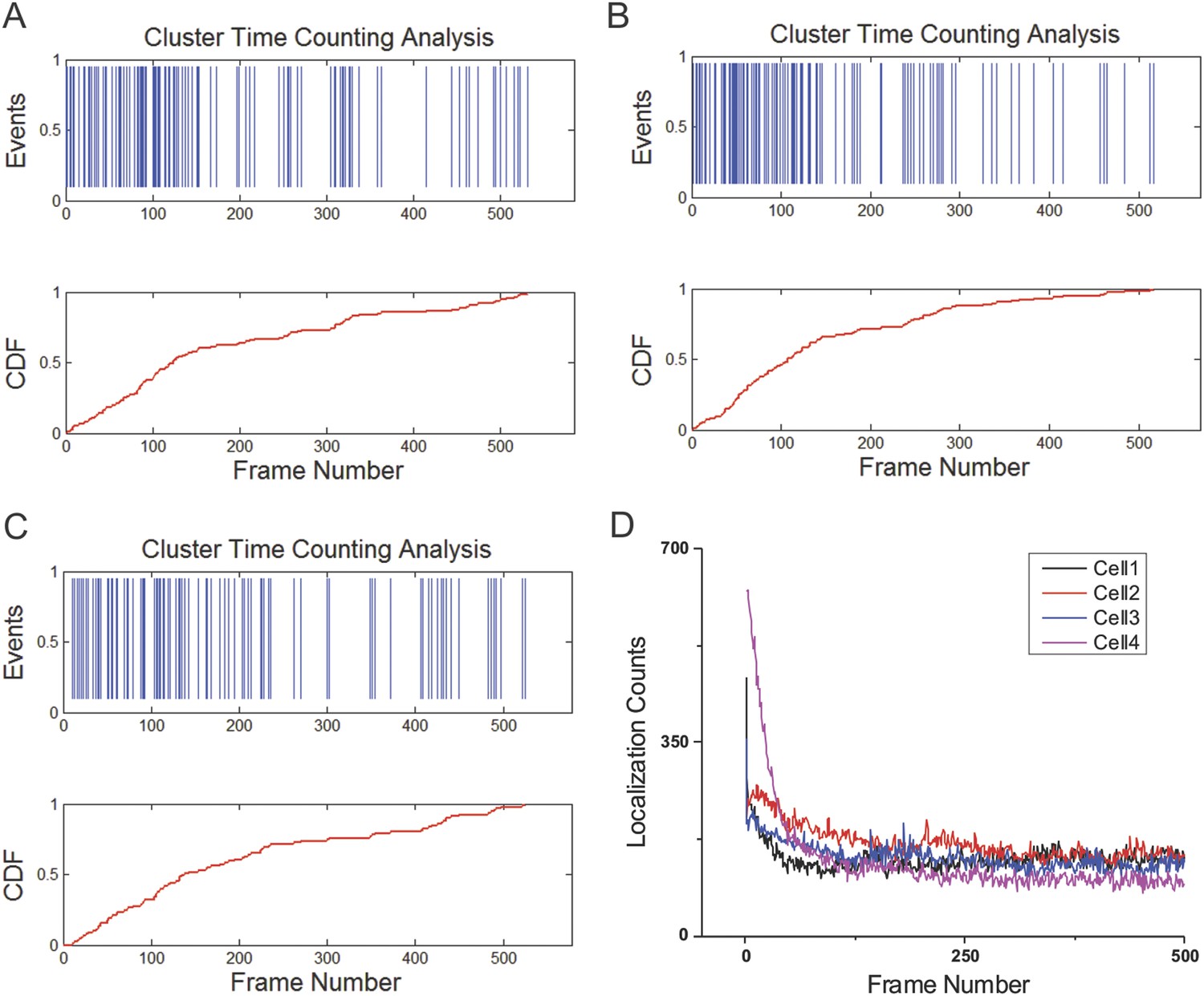
Temporal profiles of individual clusters and the number of localization detections per frame.
(A–C) Time counting of the arrival events of Sox2 stable binding sites within individual clusters. Cumulative Density Function is plotted as the function of the frame number. The time interval between two frames is 3 s. (D) To test whether photo-bleaching plays a dominant role in our imaging strategy, the number of 3D localization detections is plotted as a function of the Frame Number. The time interval between two frames is the same as in (A–C).
Figure 3 with 2 supplements
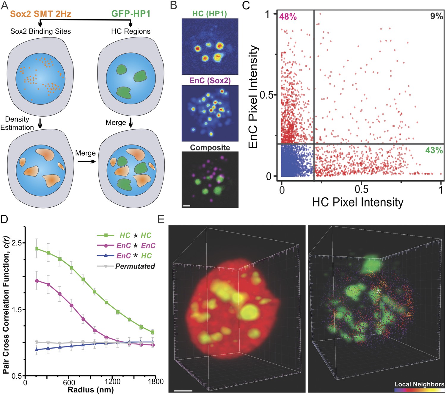
Sox2 enhancer clusters and heterochromatin regions are not co-localized.
(A) Two color imaging to probe the spatial relationship between enhancer clusters and heterochromatin regions. Sox2 stable binding sites were mapped by low-excitation 2D single molecule imaging condition (Video 7). 2D kernel density estimator was used to generate the 2D intensity map of enhancer clusters in the nucleus (Figure 3—figure supplement 1B). The intensity map of heterochromatin regions was obtained by using the GFP-HP1 channel (Figure 3—figure supplement 1A). The composite image was constructed by merging the two intensity maps as two separate color channels. (B) Single-cell exemplary images of the HC, EnC intensity maps, and the composite. See Figure 3—figure supplement 1C for more examples. (C) The pixel-to-pixel intensity plot from the HC and EnC intensity maps shown in (B). The x, y value of each point is the intensity of HC (x) and that of EnC (y) from the same pixel. Pixels with low Sox2 EnC and HC intensity values were considered as background signals (blue points). The percentile of points in each quarter (over the total number of red points) was indicated in the corner of the region. (D) Pair auto- and cross-correlation function of HC (auto, green), EnC (auto, pink), HC EnC (blue), and permutated (gray) images to investigate the spatial relationship between HC and EnC regions in single cells. , denotes the cross-correlation operator. See Equations 8–9 for calculation details. Permutation was performed by randomizing pixels spatially within the nucleus mask for both HC and EnC images prior to calculating the cross-correlation function. (E) 3D spatial relationship between heterochromatin regions and Sox2 enhancer clusters determined by two color lattice light-sheet imaging. The HaloTag-Sox2 over-labeled image (left) shows fluorescent intensities contributed by all JF549-HaloTag-Sox2 molecules and the single-molecule tracked image (right) only shows the stable Sox2 binding site distribution. See Videos 1, 8, and 9 for the exemplary raw data and the full rotation movie.
Figure 3—figure supplement 1
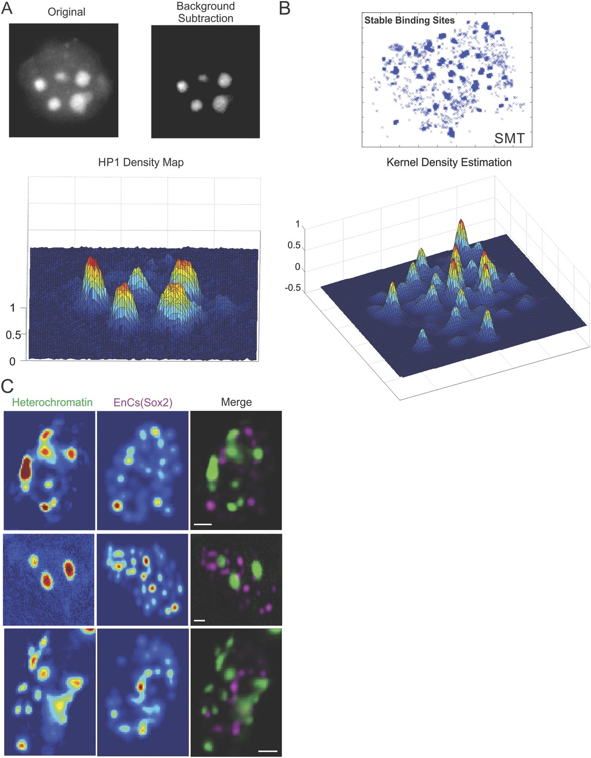
Heterochromatin and Sox2 EnC spatial relationship.
(A) Wide-field GFP-HP1 image was first processed by Matlab function to subtract background signals. Then, the normalized intensity map of heterochromatin was calculated (See details in ‘Materials and methods’ and Video 7). (B) 2D localized stable binding events (residence time > 2 s) were used for intensity estimation by a customized 2D kernel density estimator (See details in ‘Materials and methods’). (C) The intensity map of heterochromatin and that of the Sox2 enhancer clusters were used to generate the composite image on the right. Data from three cells were shown. Scale bar: 2 µm.
Figure 3—figure supplement 2
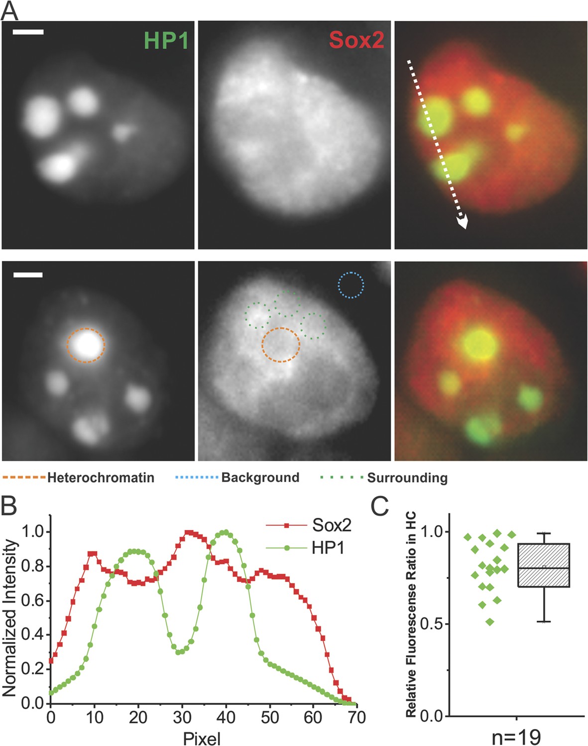
Probing Sox2 levels in heterochromatin regions.
(A) Wide-field fluorescent images of GFP-HP1, over-labeled JF549-HaloTag-Sox2, and merged from single live cells. Upper: intensity profiles from the two separate channels along the indicated path were plotted in (B). Sox2 intensity drops were observed in heterochromatin regions. Lower: the relative Sox2 intensity levels in the heterochromatin regions were compared with surrounding regions by Equation 16. The resulting ratios (n = 19 regions) were plotted in (C). Scale bar: 2 µm.
Figure 4 with 1 supplement

Sox2 targets a subset of Pol II-enriched regions in the nucleus.
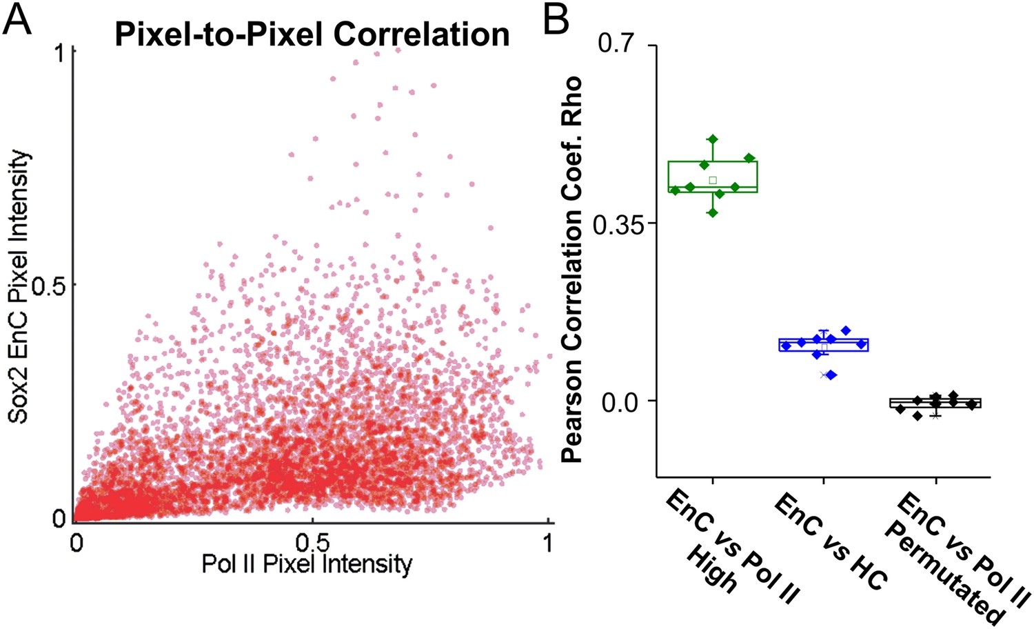
(A) Upper left: a live-cell 2D PALM super-resolution image of Dendra 2 Pol II. Upper Right: Sox2 enhancer clusters mapped by time-resolved, 2D single-molecule imaging/tracking. Stable binding events (>2 s) were shown. The color map that reflects number of local neighbors was displayed at the bottom right corner of each image. The canopy radius for calculation is 400 nm. Lower: the superimposed image of Pol II and Sox2 EnCs; Scale bar: 2 µm. (B) Selected zoomed-in views from (A); only a subset of Pol II enriched regions are targeted by Sox2. (C) Upper: single-cell exemplary images of the Pol II and EnC intensity maps calculated by 2D kernel density estimation. Lower: pair auto- and cross-correlation function of Pol II (auto, green), EnC (auto, pink), Pol II EnC (blue), and permutated (gray) images to investigate the spatial relationship between Pol II enriched and EnC regions in single cells. , denotes the cross-correlation operator. See Equations 8–9 for calculation details. Permutation was performed by randomizing pixels spatially within the nucleus mask for both Pol II and EnC images before calculating the cross-correlation function.
Figure 4—figure supplement 1
Spatial correlation between Sox2 EnCs and Pol II enriched regions.
(A) Left: the representative pixel-to-pixel intensity plot calculated from Pol II and EnC intensity maps shown in (B). Right: Pearson correlation coefficients calculated from the pixel-to-pixel correlation of Sox2 EnC & Pol II high regions (nucleolus and heterochromatin regions excluded, green), Sox2 EnC & HC (Blue), and EnC & Pol II permutated (Black) intensity plots. Please see the left panel (Pol II & EnC) and Figure 3C (HC & EnC) for representative pixel-to-pixel intensity plots.
Figure 5 with 1 supplement
Two-color imaging reveals differential Sox2 behavior within enhancer clusters vs heterochromatin.
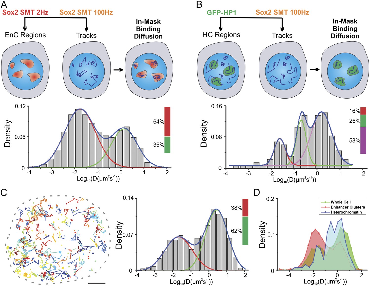
(A) Two color single-molecule imaging to probe Sox2 binding and diffusion dynamics in enhancer clusters. EnC regions were first mapped by the low-excitation, long-acquisition time condition. Then, the diffusion coefficient histogram of tracks within the EnC regions was calculated and displayed in the lower panel (n = 6 cells). See Figure 5—figure supplement 1A and Video 10 for more details. The obtained histogram was well fitted with two Gaussian peaks to a fast diffusion (green, D = 1.4 ± 0.18 μm2s−1) and a bound (red, D = 0.017 ± 0.006 μm2s−1) population. (B) Two color imaging to characterize Sox2 binding and diffusion dynamics in heterochromatin regions. Heterochromatin regions were first mapped by using the HP1-GFP marker. Then, the diffusion coefficient histogram of tracks within the heterochromatin regions was calculated and displayed in the lower panel (n = 9 cells). See Figure 5—figure supplement 1B and Video 11 for more details. The histogram was well fitted with three Gaussian peaks to a fast diffusing (pink, D = 1.58 ± 0.25 μm2s−1), a slow diffusion (green, D = 0.61 ± 0.13 μm2s−1), and a bound (red, D = 0.023 ± 0.011 μm2s−1) population. (C) Whole-cell Sox2 binding and diffusion dynamics. Single-molecule tracks were shown in the right panel. Data can be fitted by two Gaussian peaks to a fast diffusing (pink, D = 2.7 ± 0.63 μm2s−1) and a bound (red, D = 0.021 ± 0.008 μm2s−1) population (n = 12 cells). Scale bar: 2 µm. (D) Histograms from (A–C) were overlaid.
Figure 5—figure supplement 1
Regional specific diffusion and binding dynamics.
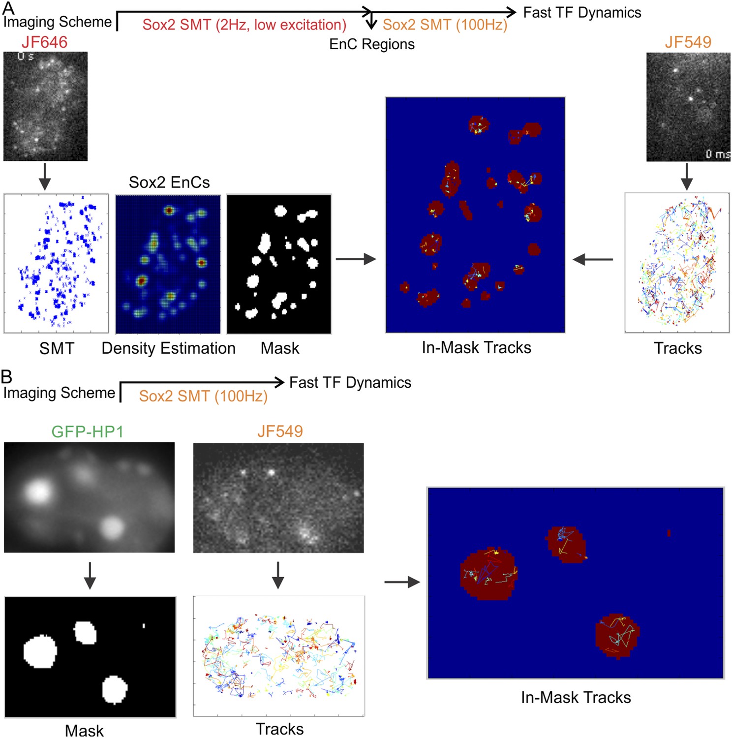
(A) Enhancer cluster regions were first mapped by low excitation, long acquisition (2 Hz) imaging of JF646-HaloTag-Sox2. Single-molecule stable binding localization events were used to generate the density intensity map by 2D kernel density estimation and the binary EnC mask was obtained by thresholding. Single-molecule tracks were generated by using the information from a fast acquisition (100 Hz) imaging condition. Tracks were divided to in-mask and out-mask fragments. Diffusion coefficients of in-mask tracks were calculated (See details in ‘Materials and methods’ and Video 10). (B) Heterochromatin regions were first mapped by using the HP1-GFP marker. HC mask was obtained by thresholding. Single-molecule tracks were generated by using the information from a fast acquisition (100 Hz) imaging condition. Tracks were divided to in-mask and out-mask fragments. Diffusion coefficients of in-mask tracks were calculated (See details in ‘Materials and methods’ and Video 11).
Figure 6 with 2 supplements

Enhancer clustering modulates global search efficiency and uncouples target search to a long-range and a local component.
(A) Monte Carlo simulation of TF target search in the nucleus to test the effects of target site distribution on the first passage 3D time (τ3D). Fold of Delay is defined as the ratio of the average τ3D in the clustered case to the average τ3D in the uniform case. In this experiment, the TF injection site is randomly selected in the nucleus with no overlap with targets. The degree of clustering is tuned by changing the indicated S.D. of the Gaussian distribution. See ‘Materials and methods’ for detailed simulation parameters. TF target search simulation experiments were performed independently 100 times of total 10 repeats for assessing the standard deviation. The Fold of Delay was plotted as a function of S.D. (Sigma) in the lower panel. (B) Monte Carlo simulation of TF target search in the nucleus to test the effects of releasing Radius (Kaur et al.) on the first passage 3D time (τ3D). The injection site is randomly constrained in a shell with the indicated releasing radius relative to the center of the cluster. Fold of Delay is defined same as in (A). TF target search simulation experiments were performed independently 100 times of total 10 repeats for assessing the standard deviation. The Fold of Delay was plotted as a function of Releasing Radius (Kaur et al.) in the lower panel. (C) The histogram distribution of τ3D for the indicated condition is fitted with both either the single-component (upper) or the two-component (lower) decay model (Equations 17–18). The experimental conditions were the same as (A).
Figure 6—figure supplement 1
TF 3D Brownian motion simulation.
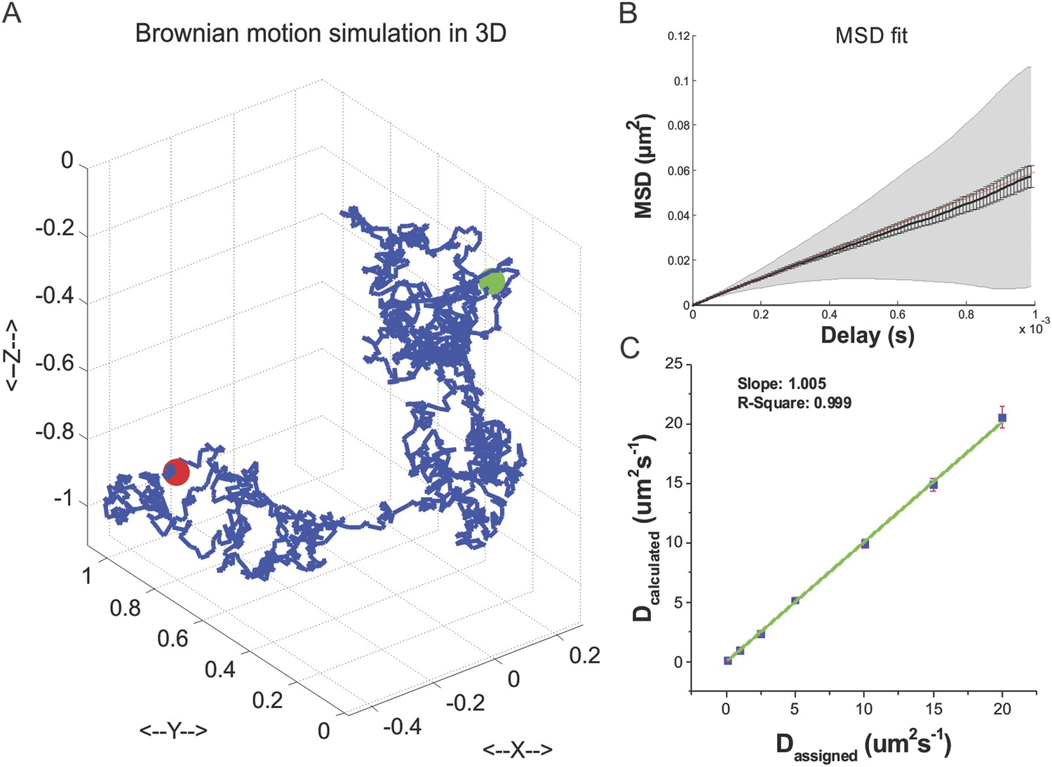
(A) An exemplary track of TF 3D Brownian motion simulated by using Equations 14–15 (See ‘Materials and methods’ for details of parameter set-ups). (B) Mean square displacement plot fitted with a linear model to extract the diffusion coefficient by MSDanalyzor. 100 simulated tracks were pooled for the calculation. (C) Validation of the Brownian motion simulation by calculating the diffusion coefficient from tracks generated by an assigned diffusion coefficient. Independent 100 tracks of total 30 repeats were used for assessing the standard deviation.
Figure 6—figure supplement 2
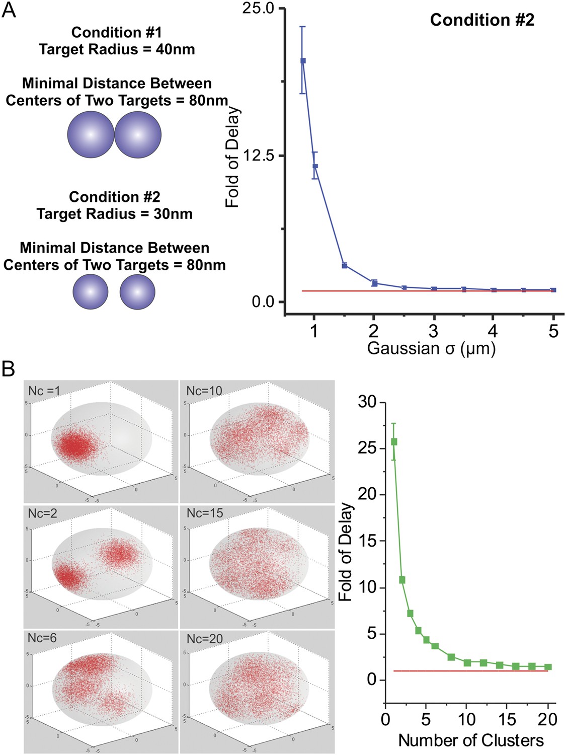
Effects of number of clusters and distance-between-targets on TF target search.
(A) To exclude the possibility that increased search times that we observed as target sites become more clustered is due to direct contacts between targets, we performed simulation experiments as described in (A) using targets with a smaller radius (30 nm) but maintained the minimal distance between targets as the same (80 nm). In the right panel, the Fold of Delay was plotted as a function of Gaussian Sigma of the sites spatial distribution. (B) Monte Carlo simulation of TF target search in the nucleus to test the effects of number of clusters (Nc) on the first passage 3D time (τ3D). Fold of Delay is defined as the ratio of the average τ3D in the clustered case to the average τ3D in the uniform case. In this experiment, the TF injection site is randomly selected in the nucleus with no overlap with targets. The targets do not overlap with each other (The minimal distance between two targets is two times of the radius of the target [80 nm]). The total number of sites remain consistent as 7000. The centers of clusters were randomly generated again for each simulation experiment. See ‘Materials and methods’ for detailed simulation parameters. TF target search simulation experiments were performed independent 100 times of total 10 repeats for assessing the standard deviation. The Fold of Delay was plotted as a function of Number of Clusters in the right panel.
Figure 7
Epigenetic perturbation of enhancer clustering and genome-wide binding.
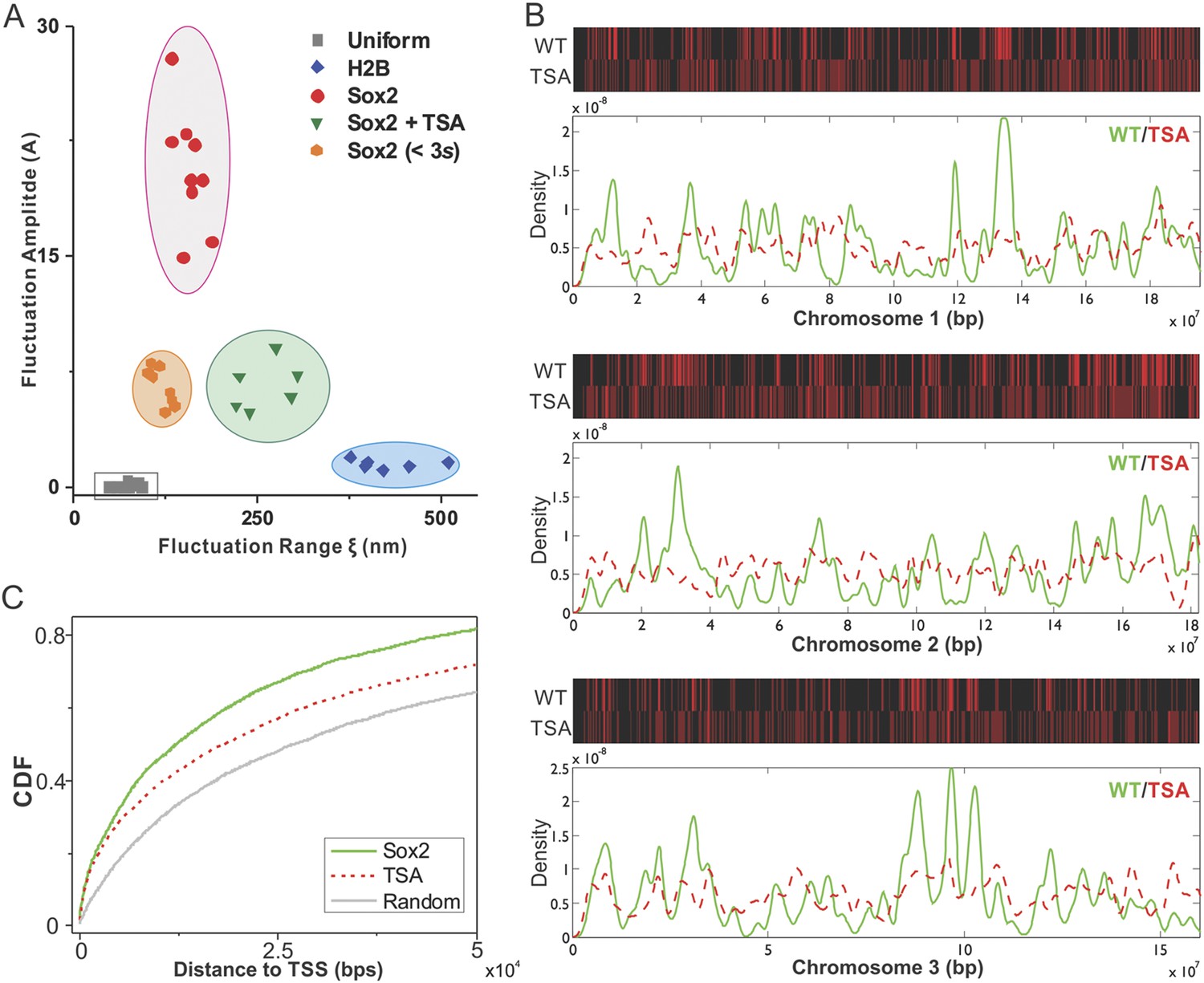
(A) The fluctuation range (x) and amplitude (y) were obtained by fitting the pair-correlation function of the indicated dataset with the fluctuation model. Figure 2 and Figure 2—figure supplement 1, Equations 10–13. Supplementary file 1. Data from the same condition were grouped in separate ellipses. (B) Sox2 ChIP-exo peak density distribution in the wild-type and TSA treated (red dotted) cells across chromosome 1, 2, 3. In the upper panels, each chromosome was divided to 500 bins. The color map correlates with the number of peaks in each bin. Top 7000 binding sites were considered in each condition. (C) Cumulative density histogram of the distances to transcription start sites (TSS's) of Sox2 ChIP-exo peaks in WT, Sox2 ChIP-exo peaks in the TSA treated cells (red dotted), and random genomic positions (gray).
Figure 8
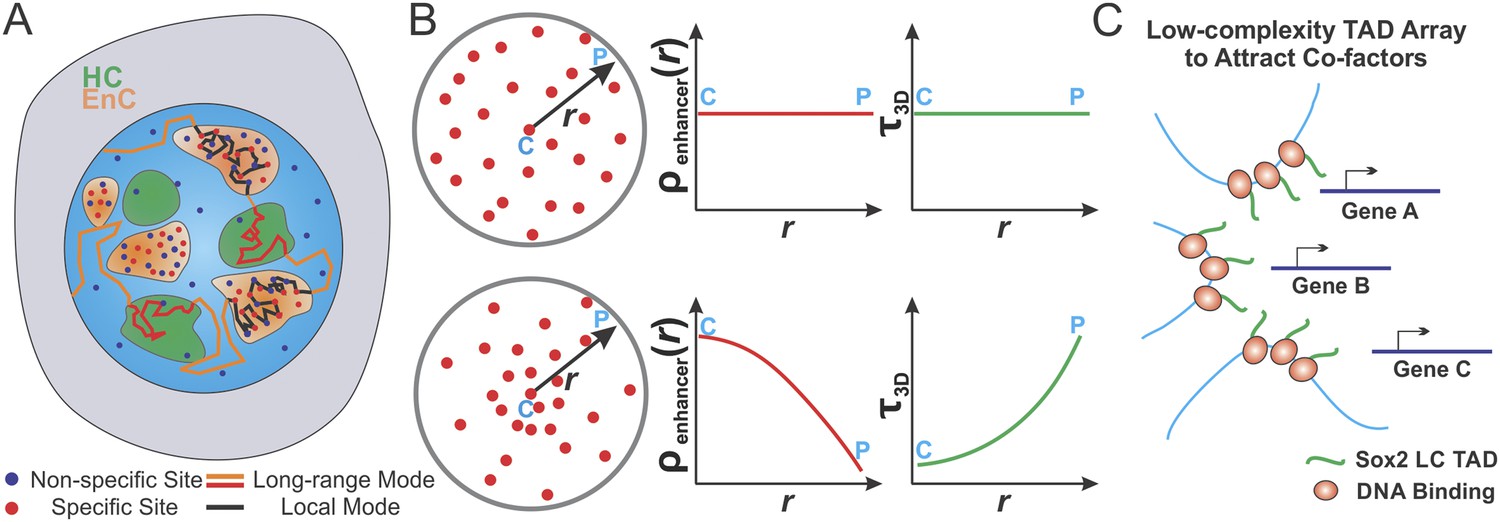
Spatially modulated target search and gene regulation in ES cells.
(A) Sox2 stable binding sites form enhancer clusters that are segregated from heterochromatin regions. Sox2 searches for targets via a 3D diffusion dominant mode traveling between clusters and tunneling through heterochromatin regions. Inside individual enhancer clusters, Sox2 3D diffusion times were dramatically shortened due to the high concentrations of specific target sites, nonspecific open DNA or protein binding partners as indicated by Figure 5A. Thus, Sox2 target search is dominated by binding processes on chromatin. (B) Enhancer clustering modulates TF target search parameters and makes spatially controlled gene regulation possible by creating variation of local enhancer concentrations. Upper, uniform distribution of target sites generates invariant enhancer site density in the nucleus and TF would have the same average 3D times across the nucleus. Lower, target site clustering causes variations of local enhancer density which would affect local target search parameters (Equations 19–21). Genes at C position would be regulated differently compared to genes at P position. C and P stand for the Center and the Peripheral, respectively. (C) Enhancer clustering promotes the formation of local Sox2 Low Complexity (LC) transactivation domain (TAD) polymer arrays which could serve as multivalent platforms to dynamically recruit co-factors for localized chromatin modulation and gene activation.
Videos
Video 1
Single-molecule light-sheet imaging of Sox2 in GFP-HP1 ES cells.
HaloTag-Sox2 is gradually labeled with JF549 ligand by diffusion. Light-sheet imaging was performed with a z step of 200 nm.
Video 2
Single-molecule, light-sheet imaging of HaloTag-Sox2 in single live ES cells.
The z step size is 300 nm.
Video 3
Reconstructed Sox2 stable binding sites in the live ES cell nucleus.
HaloTag-Sox2 stable binding sites (7000, >3 s) were localized, tracked, and reconstructed with a color map same as Figure 1C. The unit is nm. 2 cells were shown here.
Video 4
Reconstructed H2B distribution in the live ES cell nucleus.
HaloTag-H2B sites (7000) were localized, tracked, and reconstructed with a color map same as that of Figure 2A. The unit is nm.
Video 5
Uniformly distributed, simulated positions in a nucleus.
Uniformly distributed positions (7000) were presented with a color map same as that of Figure 1C. The unit is nm.
Video 6
Transient Sox2 binding sites in the live ES cell nucleus.
HaloTag-Sox2 transient binding sites (7000, <3 s) were displayed with a color map same as Figure 1C. The unit is nm.
Video 7
Map stable Sox2 binding sites in GFP-HP1 labeled cells.
Low excitation and long acquisition time (500 ms) wide-field imaging was used to map Sox2 stable binding sites in the GFP-HP1 labeled cells.
Video 8
Two color light-sheet imaging of Sox2 over-labeled GFP-HP1 ES cells.
HaloTag-Sox2 is over labeled with JF549 ligand. Light-sheet imaging was performed with a z step of 200 nm.
Video 9
3D spatial relationship between heterochromatin and Sox2 enhancer clusters.
(A) 3D reconstruction of over-labeled JF549 HaloTag-Sox2 and GFP-HP1 in single cell nucleus. (B) 3D reconstruction of JF549 HaloTag-Sox2 stable binding events (7000) (residence time >6 s) and GFP-HP1 in single cell nucleus. Scale bar, 2 µm. The color map reflects the number of local neighbors that was calculated by using a canopy radius of 400 nm.
Video 10
Tracking Sox2 binding/diffusion dynamics within enhancer clusters.
Two color single molecule imaging was performed with JF646 channel (Left) for mapping the enhancer cluster regions and JF549 (right) for tracking fast Sox2 diffusion/binding dynamics.
Video 11
Tracking Sox2 binding/diffusion dynamics in heterochromatin regions.
Two color imaging was performed with the GFP channel (upper) for mapping the heterochromatin regions and JF549 (lower) for tracking fast Sox2 diffusion/binding dynamics.
Video 12
TF target search simulation.
An example of TF target search simulation in a single nucleus.
Video 13
Reconstructed Sox2 stable binding sites in the TSA treated live cell nucleus.
HaloTag-Sox2 stable binding sites in the TSA treated live cell nucleus (7000, >3 s) were localized, tracked, and reconstructed with a color map same as that of Figure 1C. The unit is nm.
Additional files
-
Supplementary file 1
The fluctuation model fitting results, localization parameters, and ChIP-Exo primers.
- https://doi.org/10.7554/eLife.04236.033
Download links
A two-part list of links to download the article, or parts of the article, in various formats.
Downloads (link to download the article as PDF)
Open citations (links to open the citations from this article in various online reference manager services)
Cite this article (links to download the citations from this article in formats compatible with various reference manager tools)
3D imaging of Sox2 enhancer clusters in embryonic stem cells
eLife 3:e04236.
https://doi.org/10.7554/eLife.04236


