Visualizing the functional architecture of the endocytic machinery
- European Molecular Biology Laboratory, Germany
Figures
Figure 1 with 5 supplements
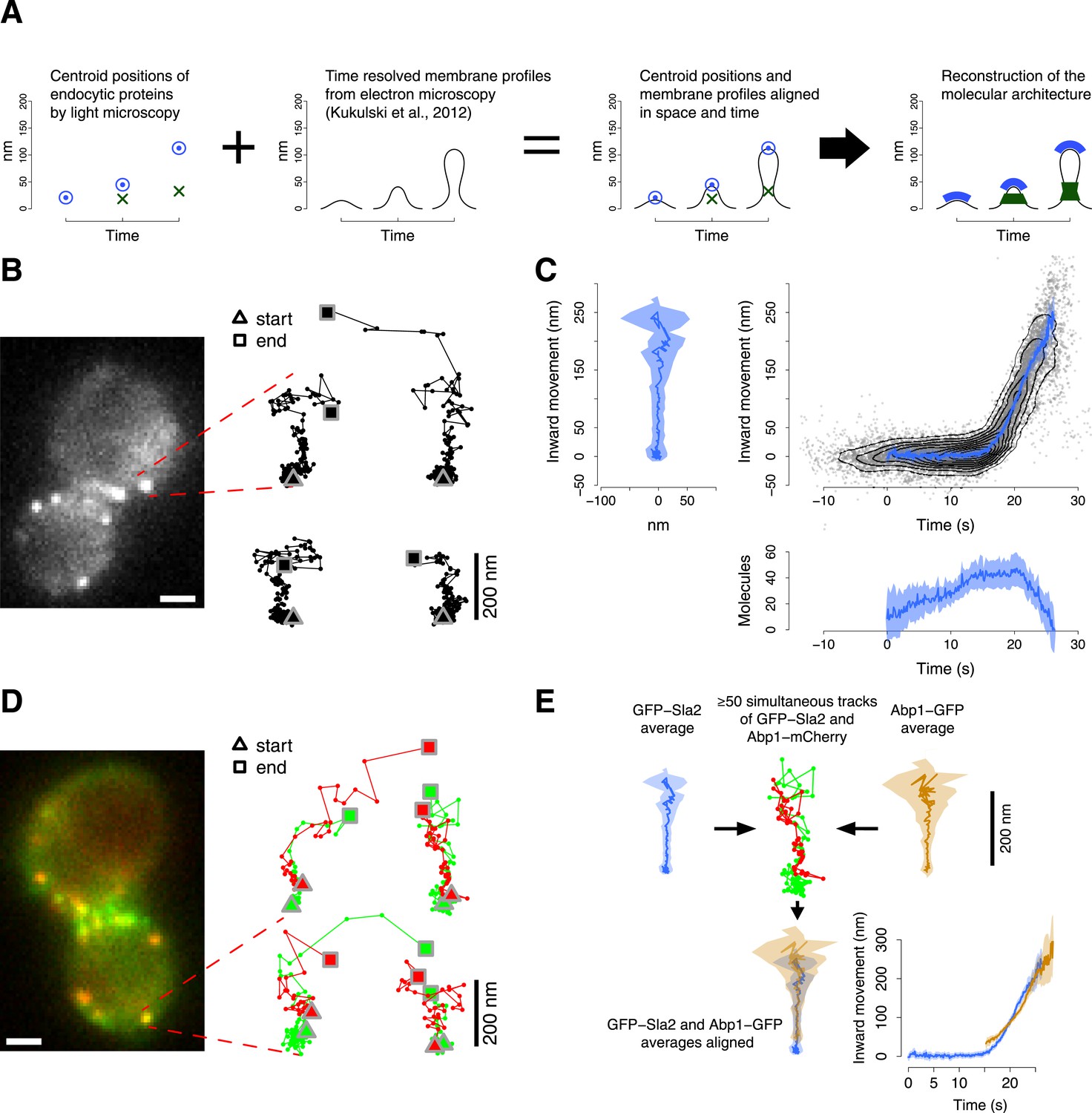
Tracking procedure.
(A) The rational behind our approach. The centroid positions of endocytic proteins were correlated with the plasma membrane intermediates derived from CLEM (Kukulski et al., 2012). We could thus position the protein complexes along the plasma membrane invagination to reconstruct the molecular architecture of the endocytic machinery. (B) A yeast cell expressing the coat protein Sla2 tagged N-terminally (GFP-Sla2) and a collection of trajectories of GFP-Sla2 centroid in different endocytic events. The trajectories are oriented so that the plasma membrane lies horizontally at the bottom and the inward movement axis is vertical. The triangle and the square mark the start and the end of each trajectory, respectively. (C) The information content of the GFP-Sla2 average trajectory: The average trajectory movement on the focal plane. The trajectory is aligned so that the Y-axis represents the inward movement along the invagination and the X-axis represents the movement along the plasma membrane (left panel). The inward movement of the trajectories over time (right panel). The number of molecules recruited at the endocytic site over time (bottom panel). The 53 individual trajectories that were used to generate this average are plotted (gray) together with the average (blue). The contour lines highlight point densities. (D) A yeast cell expressing GFP-Sla2 and the reference protein Abp1-mCherry and a collection of trajectories derived from the simultaneous acquisition of the target and reference proteins. (E) A diagram summarizing the steps that led to the spatial and temporal alignment of the average trajectories. Abp1 is used as the spatial and temporal reference. The average trajectory of the target protein (GFP-Sla2 in this example) is aligned to the average trajectory of Abp1-GFP (the reference protein) by aligning each of them to the respective trajectories acquired simultaneously in cells expressing GFP-Sla2 and Abp1-mCherry. More than 50 endocytic events are used to derive the average spatial and temporal transformation that aligns the average trajectories together. The shading represents the confidence interval (See ‘Materials and methods’). Scale bars in images are 1 µm long. See also Figure 1—figure supplements 1,2,3,4,5.
Figure 1—figure supplement 1
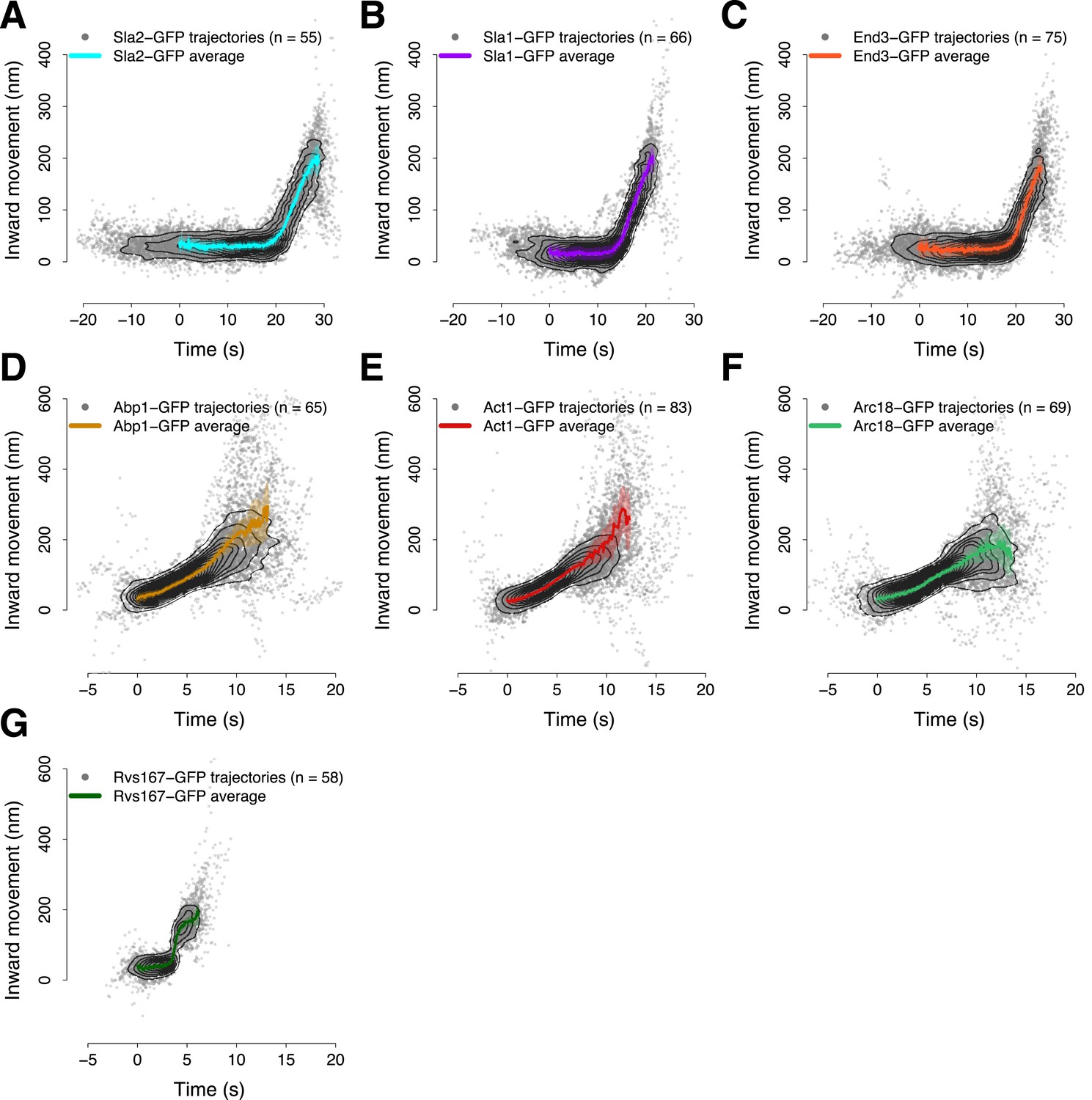
Average trajectories of endocytic events.
(A–G) The average trajectories and the individual trajectories that were used to generate the average trajectories are shown together. The contour lines highlight point densities. The distribution of the individual trajectories is unimodal confirming that the dynamics of the proteins investigated in this study do not show substantial heterogeneity during the process of endocytosis. The shading represents the confidence interval.
Figure 1—figure supplement 2
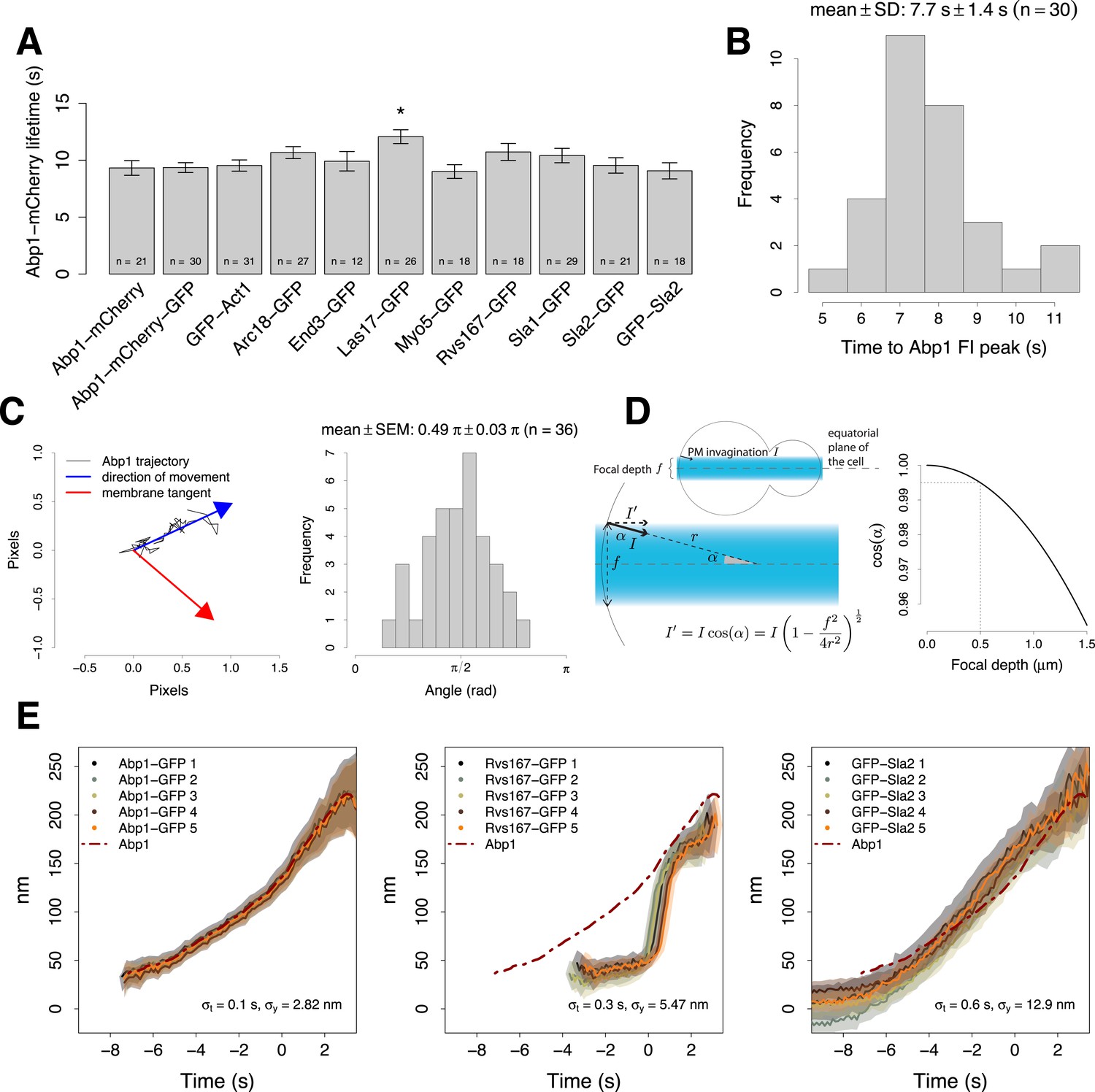
Experimental controls for the alignment procedure.
(A) Lifetimes of Abp1 patches in strains expressing Abp1-mCherry and a target protein labeled with GFP were used to control the functionality of the tagged proteins. Only Las17-GFP strain showed a significant difference in Abp1 patch lifetime (pvalue <0.05). Error bars represent the SE. (B) The time required by Abp1-GFP to reach its peak in fluorescence intensity. This gives an estimate of the time needed to invaginate the plasma membrane (Figure 2A–C). The time distribution is unimodal and normal (Shapiro–Wilk test of normality, p value = 0.07, H0: the distribution is normal.) (C) The movement of Abp1 centroid was used as a reference for the alignment of the trajectories of different endocytic proteins. Its movement is on average directed perpendicularly to the plasma membrane. The histogram shows the distribution of angles between the vector representing the direction of movement of Abp1 trajectories (blue arrow) and the vector tangent to the plasma membrane (red arrow). Mean angle is given as mean ± SEM. (D) Yeast cells were imaged at the equatorial plane therefore the invagination movement is projected on the focal plane. An endocytic event imaged at the edge of a depth of field of 500 nm (dashed lines, right plot) would induce a maximal underestimation of 0.5% of the invagination movement in a yeast cell of 2.5 μm in radius. (E) Repeated alignments of the same average trajectories (Abp1-GFP, Rvs167-GFP and GFP-Sla2) using five independent data sets of simultaneous two color acquisitions (Abp1-mCherry-GFP, Rvs167-GFP with Abp1-mCherry, and GFP-Sla2 with Abp1-mCherry). σx and σyare the standard deviations of the five alignments in time and space respectively. The shading represents the confidence interval.
Figure 1—figure supplement 3
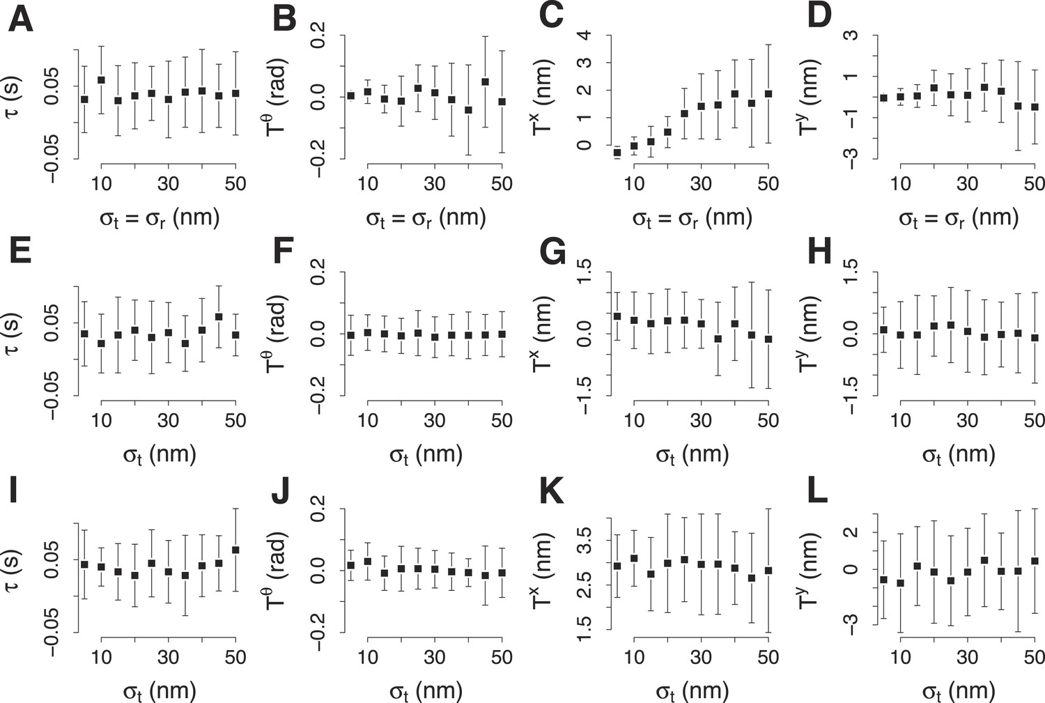
Simulation of the accuracy of the two color alignment procedure.
(A–D) Lag τ, rotation , and translations, Tx and Ty, that align a virtual trajectory to its virtual reference. The trajectory and its reference were generated already aligned and the expected values are 0 for each component of the transformation. The transformation was computed 30 times, each time using 100 trajectory pairs that were generated randomly from the virtual trajectory and the virtual reference with equal incremental values of σp and σr. σp and σr indicate respectively the standard deviation used to generate the trajectories for the target and for the reference protein in each trajectory pair. (E–H) The average values for τ, , Tx and Ty, computed as in (A–D) with incremental values of σp. σr is kept 19 nm, which is the noise we encountered experimentally for the reference trajectory in the trajectory pairs. (I–L) The average values for τ, , Tx and Ty, computed as in (E–H) but the position of the trajectory of the target protein is 30 nm away from the reference. The error bars represent the standard deviation of the distributions.
Figure 1—figure supplement 4
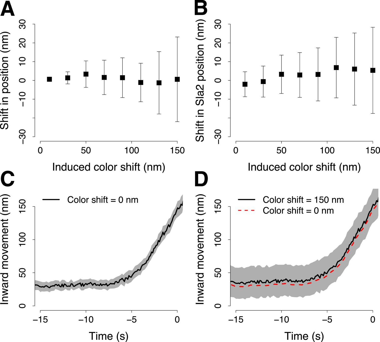
Simulation of the robustness to systematic shifts between the two channels during two color acquisition.
(A) The shift from its correct position of a trajectory aligned to its reference in the presence of systematic color aberration. Each point shows the mean and standard deviation of 30 repeats of the alignment. Each alignment was computed using 100 pairs of virtual trajectories each of which was generated with σp = 16 nm, for the trajectory of the target protein, and σr = 19 nm, for the trajectory of the reference protein. The reference trajectories were systematically shifted along one direction with incremental color shifts, which are reported along the X-axis. (B) As in (A) but with the real trajectory pairs that we acquired for Abp1-mCherry and Sla2-GFP. Those trajectory pairs were used to align Sla2-GFP to Abp1-GFP. The trajectories of Abp1-mCherry are shifted along one direction in all the trajectory pairs used to compute the alignment of Sla2-GFP. The error bars represent the confidence interval for the position of Sla2-GFP. (C–D) Examples of Sla2-GFP trajectories aligned using trajectory pairs affected by different color shifts. The shading represents the confidence interval.
Figure 1—figure supplement 5
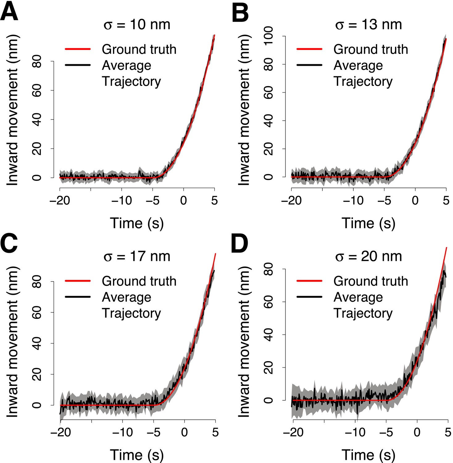
Simulation of the accuracy of the trajectory averaging.
(A) The average trajectory computed from 65 virtual trajectories that were generated from a trajectory template (ground truth trajectory, shown in red) adding noise normally distributed around the points of the ground truth trajectory with σ = 10 nm. The trajectories were aligned in space and time to compute the averaged together. The average trajectory was then aligned to its reference using 100 trajectory pairs that were generated from the ground truth trajectory, with noise σp = 10 nm and from the reference trajectory, with noise σr = 19 nm. The average trajectory is compared with the ground truth trajectory shown in red, after the alignment. (B–D) Same as (A) but with σ = 13 nm, σ = 17 nm and σ = 20 nm respectively. The shading represents the confidence interval.
Figure 2
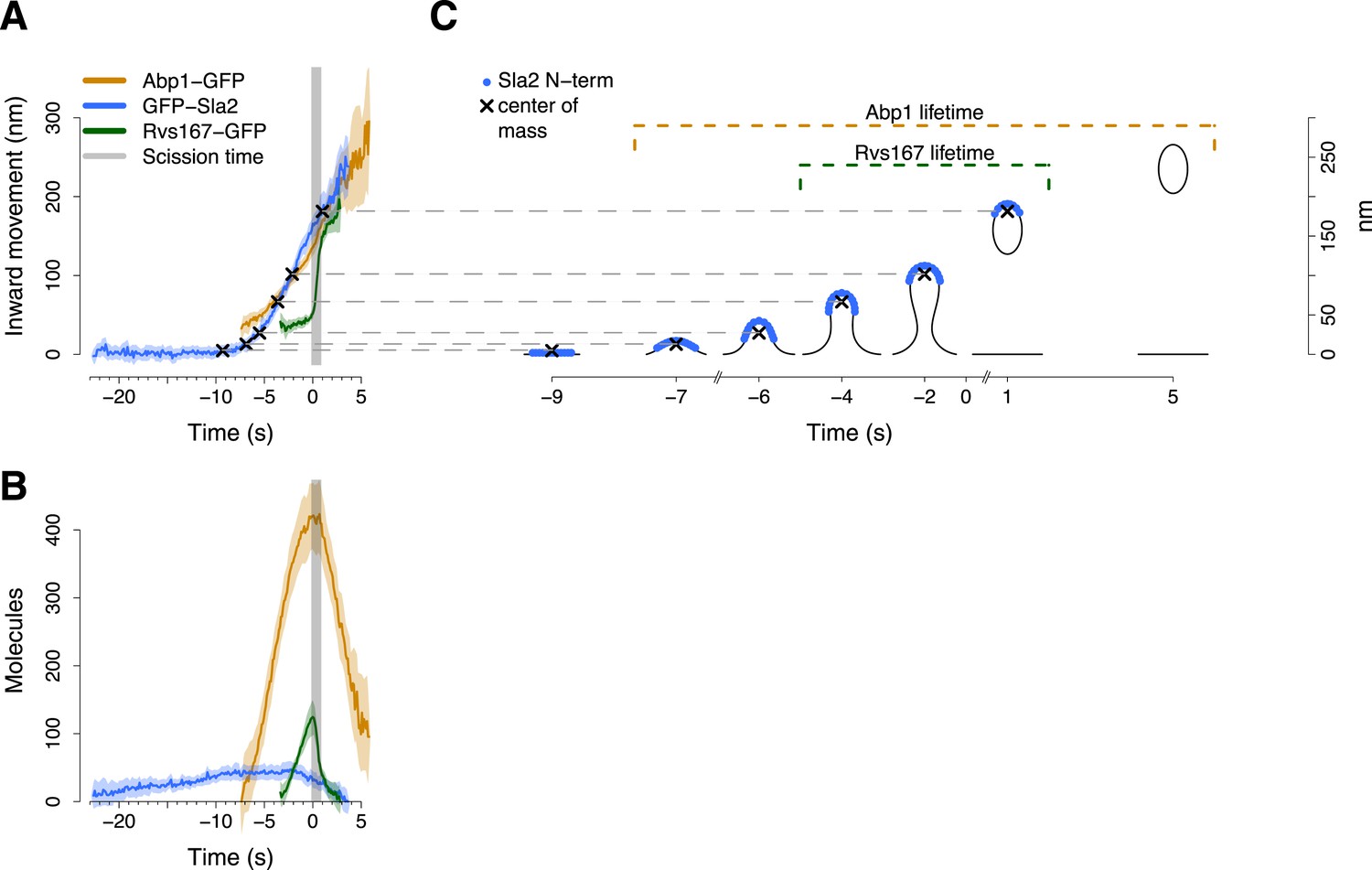
Alignment of trajectories and interpretation.
(A) Abp1-GFP, GFP-Sla2 and Rvs167-GFP average trajectories aligned with each other. (B) The average number of molecules recruited at the endocytic locus varies from protein to protein, ranging from ∼40 molecules at the peak of GFP-Sla2 to ∼410 molecules at the peak of Abp1-GFP. (C) The lifetime of Abp1-GFP and Rvs167-GFP, as well as the centroid position of GFP-Sla2 are used to align in space and time the average plasma membrane profiles obtained by correlative light and electron microscopy (Kukulski et al., 2012). The centers of mass of the Sla2 model are marked by an ‘X’. The grey vertical bar represents the estimated time window during which scission happens (Kukulski et al., 2012). The shading represents the confidence interval. The trajectories plotted are listed in Supplementary file 1.
Figure 3 with 2 supplements

Coat dynamics and organization.
(A) Left panel: the inward movement of Sla2 coat protein, tagged at its N- or C-terminus (GFP-Sla2 and Sla2-GFP respectively). Right panel: our model of Sla2 organization at the tip of the plasma membrane invagination. The centers of mass of the Sla2 model are marked by an ‘X’ (N-terminus) and an open circle (C-terminus). (B) Left panel: the inward movement of Sla1-GFP and End3-GFP. GFP-Sla2 (dashed line) is plotted for comparison. Right panel: our model of Sla1 and End3 organization at the outer rim of the coat. An open circle and an open diamond mark the centers of mass of the Sla1 and End3 models respectively. The center of mass of Sla2 N-terminus is marked by an ‘X’ and it is plotted for comparison. (C) The average number of molecules for GFP-Sla2, Sla2-GFP, Sla1-GFP and End3-GFP. (D) Sla1 ring structures imaged at endocytic sites, using superresolution microscopy. (E) Sla1 ring structures imaged at endocytic sites, using superresolution microscopy, in yeast cells treated with LatA. The shading of the trajectories represents the confidence interval. The plotted trajectories are listed in Supplementary file 1. Scale bar is 100 nm long. See also Figure 3—figure supplement 1 and Figure 3—figure supplement 2.
Figure 3—figure supplement 1
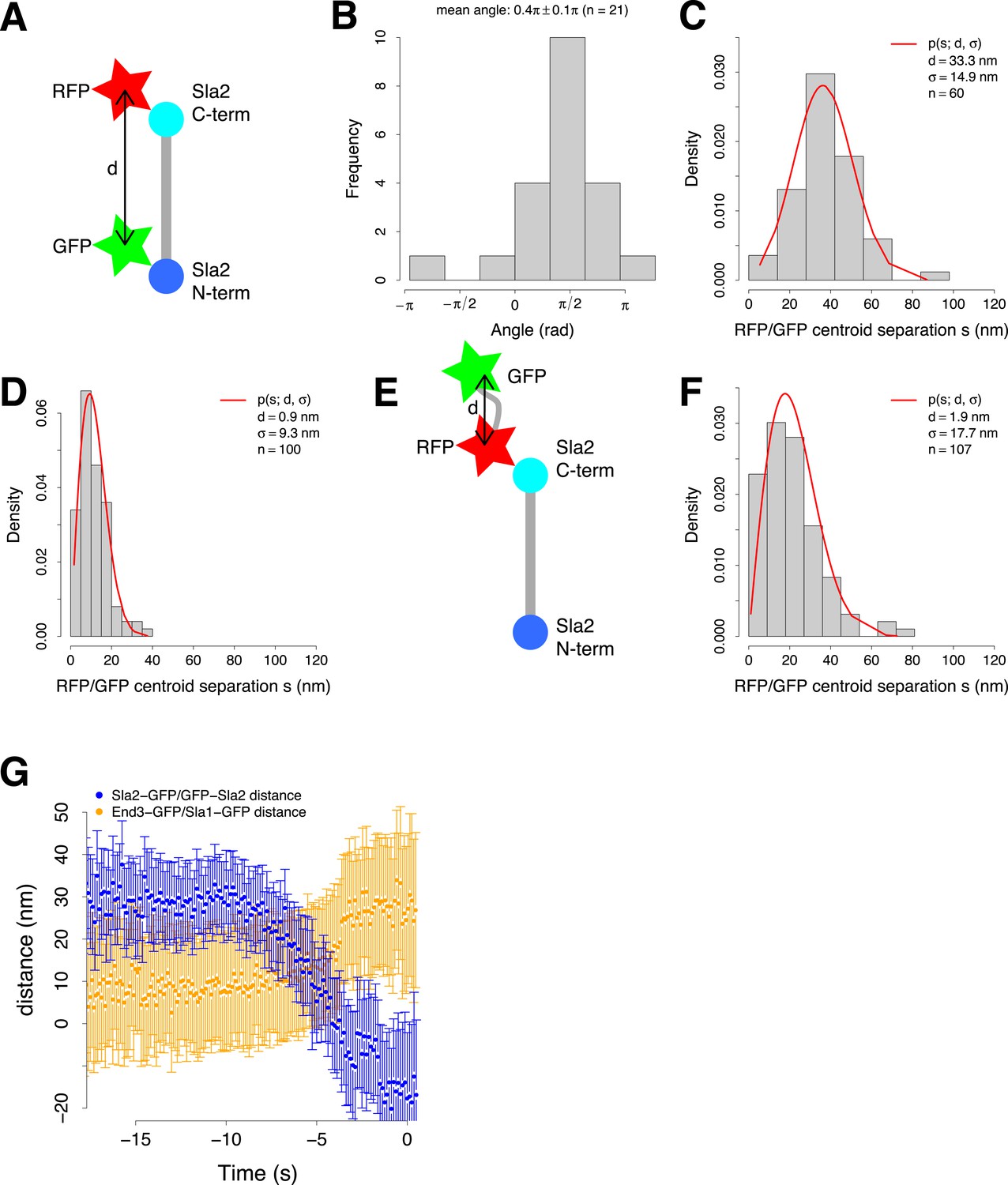
Organization of the coat and experimental control for the two color alignment.
(A) Sla2 N- and C-termini were tagged simultaneously with green (GFP) and red (RFP) fluorescent proteins respectively (GFP-Sla2-RFP). The estimated distance d between the GFP and RFP centroids gives an estimate of Sla2 length. (B) The orientation of GFP-Sla2-RFP molecules at endocytic sites in LatA treated cells. The histogram shows the angles between the vectors determined by the GFP and mCherry centroid pairs and their closest tangent to the plasma membrane. Mean angle is given as mean ± SEM. (C) The distribution of the distances s between the centroids of the N- and C-terminal tags of GFP-Sla2-RFP, measured from cells treated with LatA. The red curve marks the non-gaussian distribution that the distances follow and which is used to determine the distance d and σ (Stirling Churchman et al., 2006). (D) The distribution of the distances between centroids of TetraSpecks emitting on both GFP and mCherry channels. The red curve marks the non-gaussian distribution that the distances follow and which is used to determine d and σ (Stirling Churchman et al., 2006). (E) As an additional control the C-terminus of Sla2 was tagged with both red and green fluorescent protein in tandem (Sla2-RFP-GFP). (F) The distribution of the distances between Sla2-RFP-GFP centroids. The red curve marks the non-gaussian distribution that the distances follow and which is used to determine d and σ (Stirling Churchman et al., 2006). (G) The distance between Sla2-GFP and GFP-Sla2 average trajectories and the distance between End3-GFP and Sla1-GFP average trajectories over time. The error bars represent the confidence interval.
Figure 3—figure supplement 2
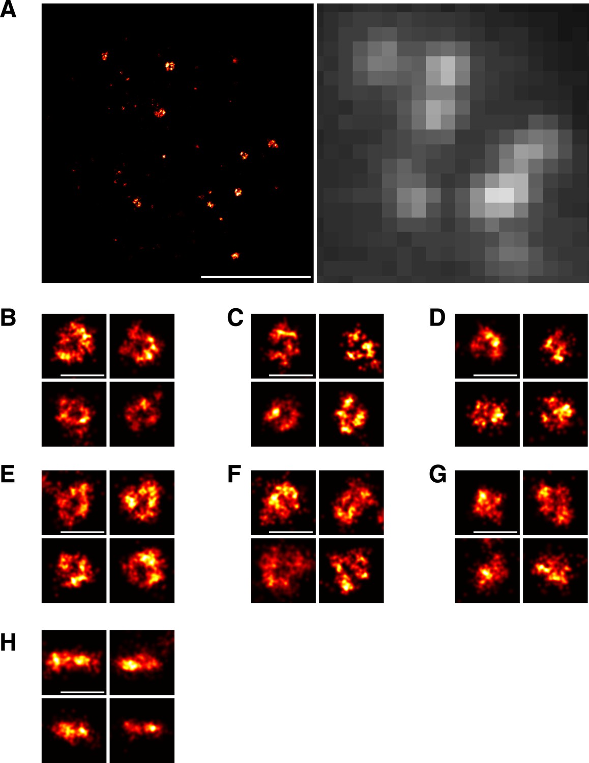
Imaging of Sla1 assemblies by localization microscopy.
(A) Overview of a yeast cell expressing Sla1-SNAP imaged using localization microscopy (left) and conventional, diffraction-limited wide-field microscopy (right). The dashed lines represent the cell outline. (B–D) We observed structural heterogeneity among the Sla1 assemblies. In addition to clear ring-shaped structures (B), a subset of Sla1 sites was found in more diverse and irregular shapes that we classified as possible rings (C) and not rings (D) (See Materials and methods). (E–G) Yeast cells expressing Sla1-SNAP were treated with LatA and imaged using localization microscopy. Similar distribution of clear ring-shapes (E), possible rings (F) and not rings (G) was observed. (H) Yeast cells expressing Sla1-SNAP and treated with LatA were imaged on the equatorial plane of cells to obtain a side view of Sla1 structures. Scale bars are 1 µm (A) and 100 nm (B–H).
Figure 4 with 1 supplement
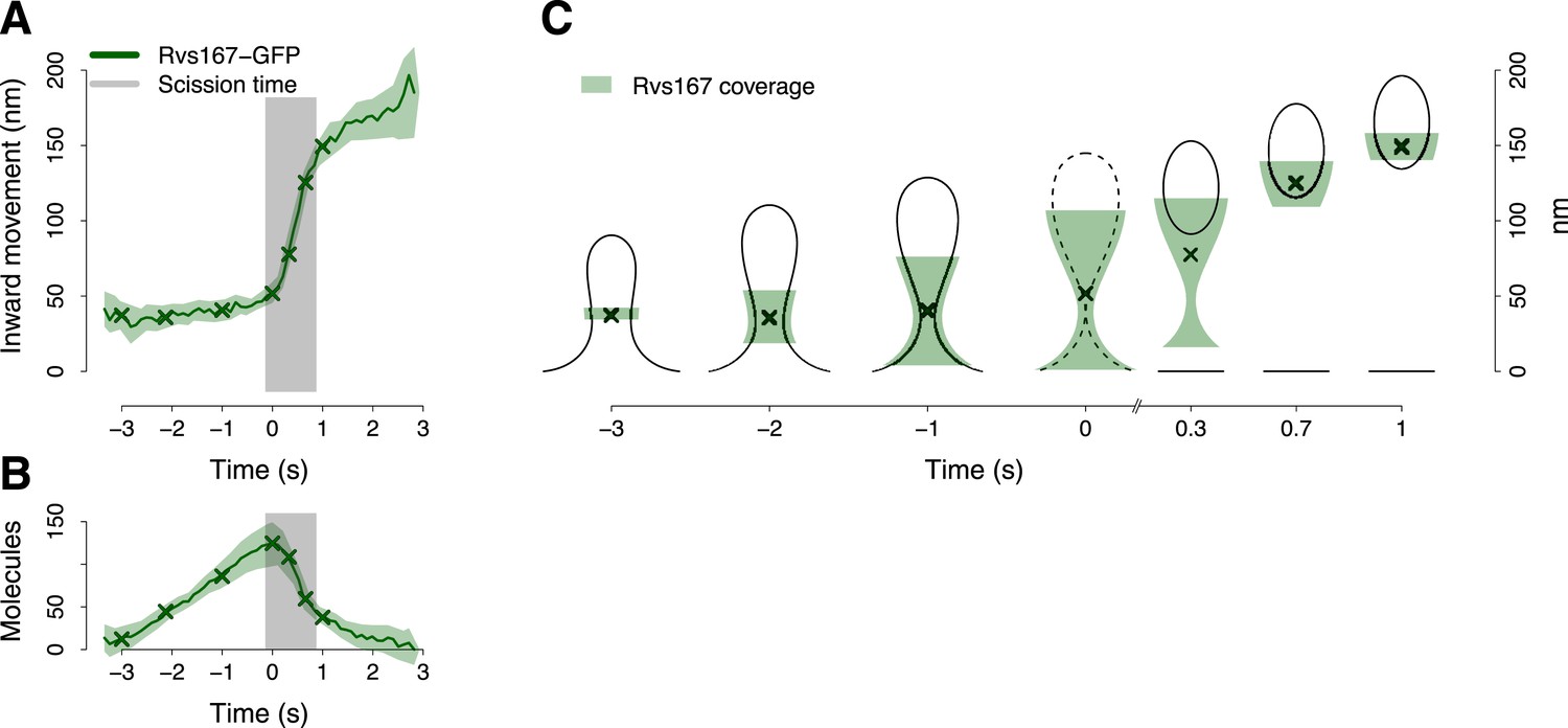
BAR protein dynamics.
(A) The inward movement of Rvs167-GFP. (B) The average number of molecules of Rvs167-GFP. (C) Our model of Rvs coverage of the plasma membrane invagination during the invagination growth. When scission happens, Rvs molecules are released rapidly and remain in proximity of the vesicle only. The centers of mass of the Rvs model are marked by an ‘X’. The grey vertical bar represents the estimated time window during which scission happens (Kukulski et al., 2012). The shading represents the confidence interval. The plotted trajectories are listed in Supplementary file 1. See also Figure 4—figure supplement 1.
Figure 4—figure supplement 1
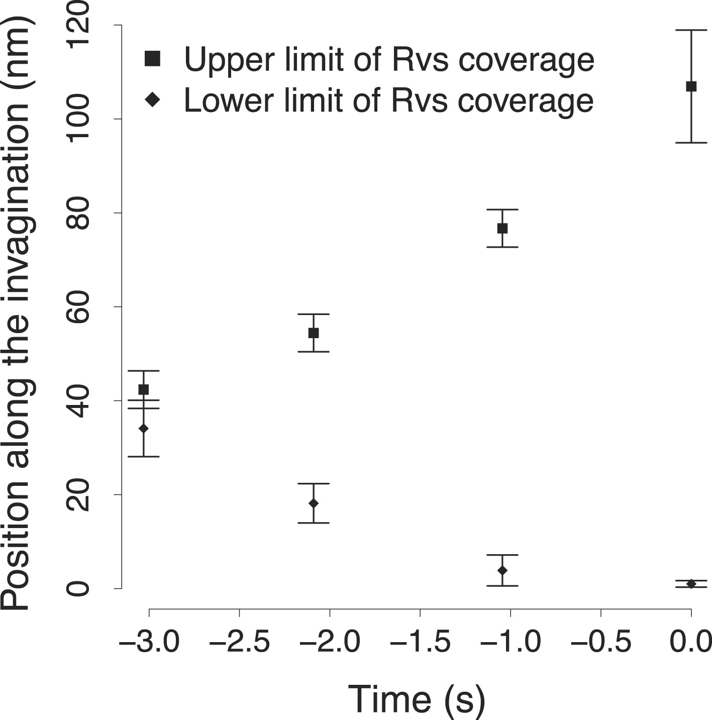
The variability in the BAR protein coverage of the plasma membrane.
The points show the upper and lower bound of the Rvs coverage shown in Figure 4C. The error bars show the variability in the calculation of the extent of Rvs coverage of the plasma membrane as a function of the uncertainty in the number of molecules (Figure 4B).
Figure 5

Actin cytoskeleton dynamics.
(A) The inward movement of the actin cytoskeleton components GFP-Act1, Arc18-GFP and Abp1-GFP, together with the nucleation factors Las17-GFP and Myo5-GFP. GFP-Sla2 (dashed line) is plotted for comparison. (B–C) The average number of molecules of Las17-GFP, GFP-Act1, Myo5-GFP, Abp1-GFP and Arc18-GFP. The grey vertical bar represents the estimated time window during which scission happens (Kukulski et al., 2012). The shading represents the confidence interval. The plotted trajectories are listed in Supplementary file 1.
Figure 6 with 1 supplement
Region of assembly of actin filaments.
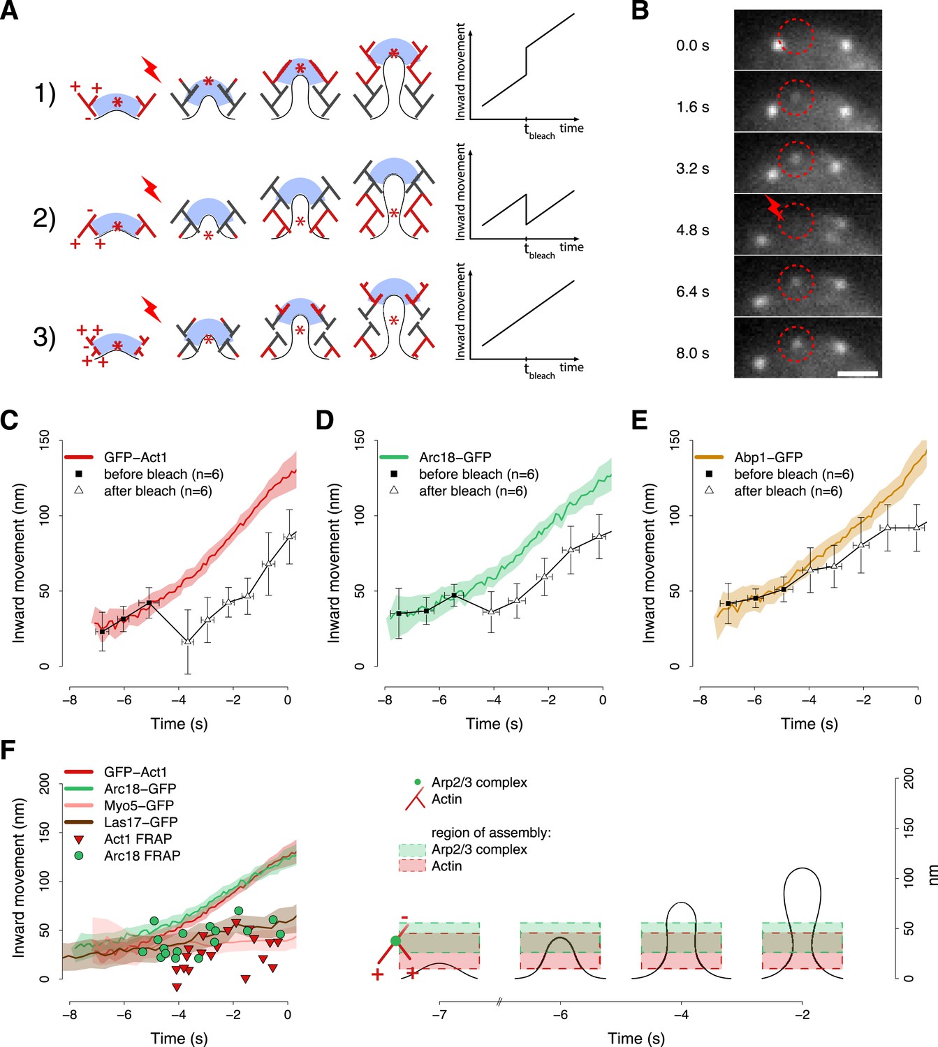
(A) A schematic cartoon to show how local photobleaching would affect the centroid position of a fluorescent actin patch, given three possible scenarios for the nucleation of new actin filaments (in red) at the endocytic locus: (1) New actin filaments are nucleated in the proximity of the coat; photobleaching would shift the centroid away from the plasma membrane. (2) New filaments are nucleated at the base of the plasma membrane invagination; photobleaching would shift the centroid toward the plasma membrane. (3) There is no preferential direction for actin nucleation; photobleaching would not affect the centroid position. (B) Local photobleaching of an endocytic event in a cell expressing GFP-Act1. Scale bar: 1 μm. See also Video 1. (C–E) Centroid positions of endocytic patches in yeast cells expressing GFP-Act1 (C), Arc18-GFP (D) or Abp1-GFP (E) before and after photobleaching. Error bars represent the Standard Deviation. Plots show the respective average trajectories for comparison. (F) Left panel: The locations of the first post-bleach centroids of Act1-GFP (red triangles) and Arc18-GFP (green circles) aligned relative to the unbleached average trajectories. Nucleation promoting factors, Myo5-GFP and Las17-GFP, localize to the same region where actin monomers are added. Average trajectories of GFP-Act1 and Arc18-GFP are plotted for comparison. Right panel: Our model for the region of actin polymerization. The dashed boxes highlight the region where actin and Arp2/3 complexes are recruited. The centers and the heights of the boxes correspond respectively to the average and to the standard deviation of the centroid positions of GFP-Act1 and Arc18-GFP after photobleaching. The cartoon highlights the regions where the new Arp2/3 complexes and actin molecules are recruited. The shading of the trajectories represents the confidence interval. The plotted trajectories are listed in Supplementary file 1. See also Figure 6—figure supplement 1.
Figure 6—figure supplement 1
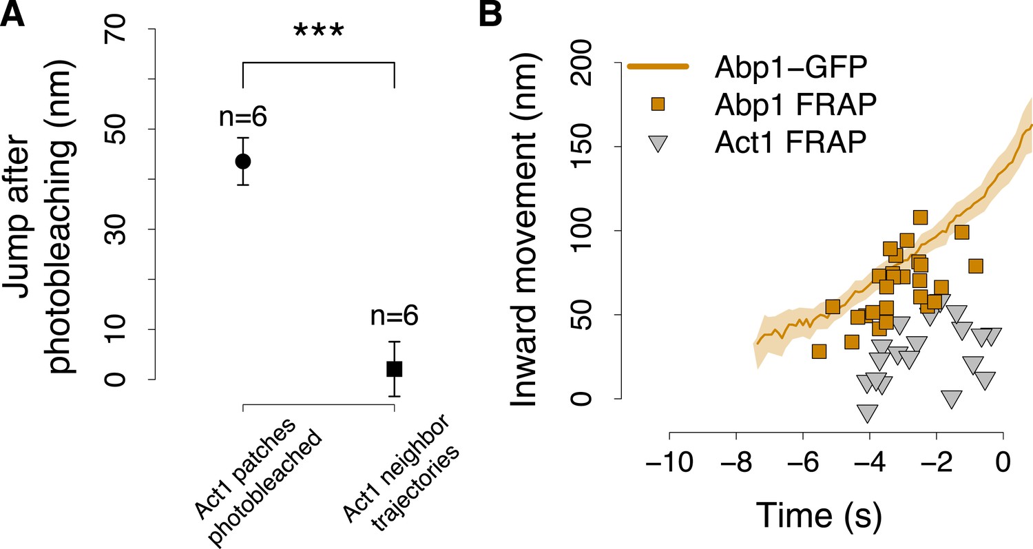
The position of Abp1 fluorescence recovery after photobleaching.
(A) The quantification of the jump in GFP-Act1 patches photobleached 3–4 s after the appearance of the patch (data showed in Figure 6C), compared with the jump in GFP-Act1 patches that where next to the region photobleached and thus were only partially affected by the photobleaching. Error bars represent the SEM. (B) The centroid positions of endocytic fluorescent patches recovering after photobleaching (FRAP), performed at different time points during the plasma membrane invagination process, in yeast cells expressing Abp1-GFP. The shading represents the confidence interval. GFP-Act1 FRAP are the data showed in Figure 6F and serve as a comparison.
Figure 7

The dynamic architecture of the endocytic machinery.
(A) Summary of the average dynamics and number of molecules for Sla2-GFP, GFP-Sla2, Sla1-GFP, End3-GFP, Rvs167-GFP, Arc18-GFP, Myo5-GFP, Las17-GFP and GFP-Act1. The plotted trajectories are listed in Supplementary file 1. Las17 and Myo5 were smoothened using a moving average filter of length 5; the remaining data were smoothed using a Savitzky-Golay filter over 11 time points. (B) The protein symbols are positioned, according to the average trajectories of the corresponding proteins (Figure 7A), along the plasma membrane invagination profiles derived from CLEM. The actin filament network is drawn schematically to illustrate the average direction of actin polymerization and does not represent the true organization of the actin filaments and branches. Time ≤ −8 s: coat assembly; Sla2 exposes its actin binding domain outside of the clathrin cage. Time ≈ −8 s: actin polymerization starts and drives the initiation of the plasma membrane invagination. −8 s ≤ time ≤ −3 s: the invagination grows and the coat accommodates the changes in curvature imposed by the plasma membrane invagination growth. −3 s ≤ time < 0 s: Rvs proteins are recruited to the invagination, which is growing longer, and stabilize it. Time ≥ 0: the scission of the invagination releases the vesicle. Concomitantly, the Rvs structure starts to disassemble very rapidly. See also Video 2.
Videos
Video 1
Photobleaching experiment.
Local photobleaching of an endocytic event in a cell expressing GFP-Act1. The video plays in real time. Scale bar is 2 µm.
Video 2
The dynamic architecture of the endocytic machinery.
The reconstruction of the dynamic architecture of the endocytic machinery obtained by combining the centroid positions of the proteins over time, the plasma membrane invagination profiles derived from CLEM (Kukulski et al., 2012) and the structural properties of the proteins. See also Figure 7 for the legend of the protein symbols.
Tables
Table 1
Number of trajectories used in this study
| Number of single color trajectories to generate the average trajectory | Number of trajectory pairs used for spatial and temporal alignment | |
|---|---|---|
| GFP-Sla2 | 53 | 271 |
| Sla2-GFP | 55 | 158 |
| Sla1-GFP | 66 | 58 |
| End3-GFP | 75 | 57 |
| Abp1-GFP | 65 | NA |
| GFP-Act1 | 83 | 92 |
| Arc18-GFP | 69 | 90 |
| Rvs167-GFP | 58 | 340 |
| Las17-GFP | NA | 49 |
| Myo5-GFP | NA | 50 |
| TOTAL | 524 | 1165 |
-
The number of events that were tracked and used to compute the average trajectories and to align those average trajectories together.
Table 2
Yeast strains
| Strain # | Genotype |
|---|---|
| MKY0216 | MATa, his3-∆200, leu2-3,112, ura3-52, lys2-801, NUF2-EGFP::HIS3MX6 |
| MKY0217 | MATα, his3-∆200, leu2-3,112, ura3-52, lys2-801, NUF2-EGFP::HIS3MX6 |
| MKY0711 | MATa, his3-∆200, leu2-3,112, ura3-52, lys2-801, MYO5-EGFP::HIS3MX6, ABP1-mCherry::kanMX4 |
| MKY0822 | MATa, his3-∆200, leu2-3,112, ura3-52, lys2-801, SLA1-EGFP::HIS3MX6, ABP1-mCherry::kanMX |
| MKY1304 | MATa, his3-∆200, leu2-3,112, ura3-52, lys2-801, END3-EGFP::HIS3MX6, ABP1-mCherry::kanMX4 |
| MKY1318 | MATa, his3-∆200, leu2-3,112, ura3-52, lys2-801, RVS167-EGFP::HIS3MX6, ABP1-mCherry::kanMX4 |
| MKY1368 | MATα, his3-∆200, leu2-3,112, ura3-52, lys2-801, LAS17-EGFP::HIS3MX6, ABP1-mCherry::kanMX4 |
| MKY2119 | MATα, his3-∆200, leu2-3,112∆::GalL-ISce1-natNT2, ura3-52, lys2-801, sfGFP-SLA2-mCherry::hphNT1 |
| MKY2653 | MATa, his3-∆200, leu2-3,112, ura3-52, lys2-801 with pMK0100[CEN, URA3 GFP-ACT1] |
| MKY2655 | MATa, his3-∆200, leu2-3,112, ura3-52, lys2-801, ABP1-mCherry::kanMX4 with pMK0100[CEN, URA3 GFP-ACT1] |
| MKY2689 | MATα, his3-∆200, leu2-3,112∆::GalL-ISce1-natNT2, ura3-52, lys2-801, sfGFP-SLA2 |
| MKY2720 | MATa, his3-∆200, leu2-3,112, ura3-52, lys2-801, ARC18-myEGFP::natNT2, ABP1-mCherry::kanMX |
| MKY2747 | MATa, his3-∆200, leu2-3,112, ura3-52, lys2-801, ARC18-myEGFP::natNT2 |
| MKY2832 | MATa, his3-∆200, leu2-3,112, ura3-52, lys2-801, RVS167-EGFP::HIS3MX6 |
| MKY2833 | MATa, his3-∆200, leu2-3,112, ura3-52, lys2-801, SLA1-EGFP::HIS3MX6 |
| MKY2834 | MATα, his3-∆200, leu2-3,112, ura3-52, lys2-801, ABP1-EGFP::HIS3MX6 |
| MKY2836 | MATα, his3-∆200, leu2-3,112∆::GalL-ISce1-natNT2, ura3-52, lys2-801, sfGFP-SLA2, ABP1-mCherry::kanMX |
| MKY3135 | MATα, his3-∆200, leu2-3,112∆::GalL-ISce1-natNT2, ura3-52, lys2-801, sfGFP-SLA2, ABP1-mCherry::kanMX, Sla1-SNAP::HIS3MX6 |
| MKY2859 | MATa, his3-∆200, leu2-3,112, ura3-52, lys2-801, SLA2-EGFP::HIS3MX6 |
| MKY2863 | MATa, his3-∆200, leu2-3,112, ura3-52, lys2-801, CSE4-EGFP::HIS3MX6 |
| MKY2864 | MATa, his3-∆200, leu2-3,112, ura3-52, lys2-801, LAS17-EGFP::HIS3MX6 |
| MKY2876 | MATa, his3-∆200, leu2-3,112, ura3-52, lys2-801, MYO5-EGFP::HIS3MX6 |
| MKY2880 | MATa, his3-∆200, leu2-3,112, ura3-52, lys2-801, ABP1-mCherry-sfGFP::kanMX4 |
| MKY2893 | MATa, his3-∆200, leu2-3,112, ura3-52, lys2-801, END3-EGFP::HIS3MX6 |
| MKY2918 | MATα, his3-∆200, leu2-3,112, ura3-52, lys2-801, SLA2-EGFP::HIS3MX6, ABP1-mCherry::kanMX4 |
| MKY2919 | MATa, his3-∆200, leu2-3,112∆::GalL-ISce1-natNT2, ura3-52, lys2-801, NUF2-sfGFP::KIURA3 |
| MKY2920 | MATα, his3-∆200, leu2-3,112∆::GalL-ISce1-natNT2, ura3-52, lys2-801, NUF2-sfGFP::KIURA3 |
| MKY3136 | MATa, his3-∆1, leu2-∆0, ura3-∆0, met15-∆0, LAS17-myEGFP::natNT2 |
| MKY3137 | MATa, his3-∆1, leu2-∆0, ura3-∆0, met15-∆0, RVS167-myEGFP::natNT2 |
-
The yeast strains used in this study.
Additional files
-
Supplementary file 1
Average trajectory data. The average trajectories plotted in Figures 1–6 t: time points in seconds (time 0 corresponds to the Rvs167 intensity peak). t.err: 95% confidence interval of the time alignment in seconds. x: centroid position, in respect to the plasma membrane and along the invagination axis (nm). x.err: 95% confidence interval of the centroid position, in respect to the plasma membrane and along the invagination axis (nm). n: estimate of number of molecules. n.err: 95% confidence interval of the number of molecules.
- https://doi.org/10.7554/eLife.04535.023
-
Source code 1
Average trajectories V0.1.
The collection of R functions used to compute the average trajectories. They require the R library Hmisc.
- https://doi.org/10.7554/eLife.04535.024
-
Source code 2
Align trajectories V0.2.
The collection of R functions used to align the average trajectories together and to plot them. They require the R library MASS and the function plotCI form the R package gregmisc.
- https://doi.org/10.7554/eLife.04535.025
Download links
A two-part list of links to download the article, or parts of the article, in various formats.
Downloads (link to download the article as PDF)
Open citations (links to open the citations from this article in various online reference manager services)
Cite this article (links to download the citations from this article in formats compatible with various reference manager tools)
Visualizing the functional architecture of the endocytic machinery
eLife 4:e04535.
https://doi.org/10.7554/eLife.04535


