Homeostatic reinforcement learning for integrating reward collection and physiological stability
Figures
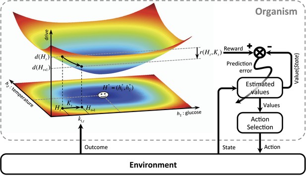
Schematics of the model in an exemplary two-dimensional homeostatic space.
Upon performing an action, the animal receives an outcome from the environment. The rewarding value of this outcome depends on its ability to make the internal state, , closer to the homeostatic setpoint, , and thus reduce the drive level (the vertical axis). This experienced reward, denoted by , is then learned by an RL algorithm. Here a model-free RL algorithm is shown in which a reward prediction error signal is computed by comparing the realized reward and the expected rewarding value of the performed response. This signal is then used to update the subjective value attributed to the corresponding response. Subjective values of alternative choices bias the action selection process.
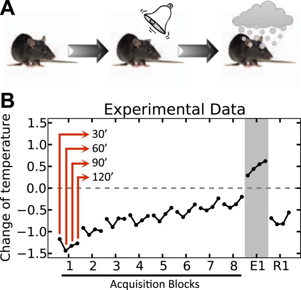
Experimental results (adapted from Mansfield & Cunningham, 1980) on the acquisition and extinction of conditioned tolerance response to ethanol.
(A) In each block (day) of the experiment, the animal received ethanol injection after the presentation of the stimulus. (B) The change in the body temperature was measured 30, 60, 90, and 120 min after ethanol administration. Initially, the hypothermic effect of ethanol decreased the body temperature of animals. After several training days, however, animals learned to activate a tolerance response upon observing the stimulus, resulting in smaller deviations from the temperature setpoint. If the stimulus was not followed by ethanol injection, as in the first day of extinction (E1), the activation of the conditioned tolerance response resulted in an increase in body temperature. The tolerance response was weakened after several (four) extinction sessions, resulting in increased deviation from the setpoint in the first day of re-acquisition (R1), where presentation of the cue was again followed by ethanol injection.
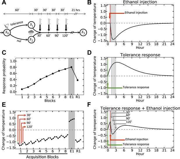
Simulation result on anticipatory responding.
(A) In every trial, the simulated agent can choose between initiating a tolerance response and doing nothing, upon observing the stimulus. Regardless of the agent's choice, ethanol is administered after 1 hr, followed by four temperature measurements every 30 min. (B) Dynamics of temperature upon ethanol injection. (C) Learning curve for choosing the ‘tolerance’ response. (D) Dynamics of temperature upon initiating the tolerance response. (E) Temperature profile during several simulated trails. (F) Dynamics of temperature upon initiating the tolerance response, followed by ethanol administration. Plots c and e are averaged over 500 simulated agents.
-
Figure 3—source data 1
Free parameters for the anticipatory responding simulation.
- https://doi.org/10.7554/eLife.04811.006
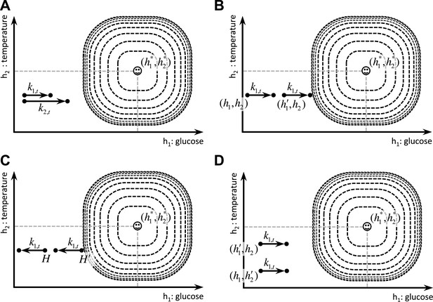
Schematic illustration of the behavioral properties of the drive function.
(A) excitatory effect of the dose of outcome on its rewarding value. (B, C) excitatory effect of deprivation level on the rewarding value of outcomes: Increased deprivation increases the rewarding value of reducing drive (B), and increases the punishing value of increasing drive (C). (D) inhibitory effect of irrelevant drives on the rewarding value of outcomes.
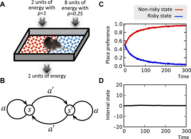
Risk aversion simulation.
In a conditioned place preference paradigm, the agent's presence in the left and the right compartments has equal expected payoffs, but different levels of risk (A) Panel (B) shows the Markov decision process of the same task. In fact, in every trial, the agent chooses whether to stay it the current compartment, or transit to the other one. The average input of energy per trial, regardless of the animal's choice, is set such that it is equal to the animal's normal energy expenditure. Thus, the internal state stays close to its initial level, which is equal to the setpoint here (D). The model learns to prefer the non-risky over the risky compartments (C) in order to avoid severe deviations from the setpoint.
-
Figure 5—source data 1
Free parameters for the risk-aversion simulations.
- https://doi.org/10.7554/eLife.04811.009
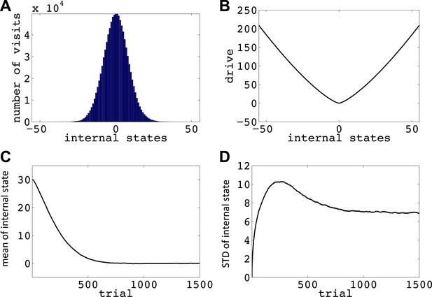
Simulations showing that the model avoids extreme deviations.
Starting from 30, the agent can either decrease or increase its internal state by one unit in each trial. (A) The number of visits at each internal state after 106 trials. (B) The drive function in the one-dimensional homeostatic space. (setpoint = 0). The mean (C) and standard deviation (D) of the internal state of 105 agents, along 1500 trials.
-
Figure 6—source data 1
Free parameters for the simulations showing that the model avoids extreme homeostatic deviations.
- https://doi.org/10.7554/eLife.04811.011

The Markov Decision Process used for simulation results presented in Figure 6 and Figure 6—figure supplements 2–7.
https://doi.org/10.7554/eLife.04811.012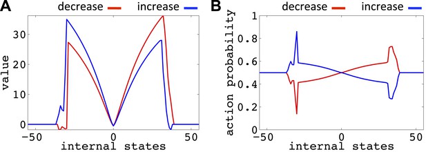
Value function (A) and choice preferences (B) for state–action pairs after simulating one agent for 106 trials (As in Figure 6).
The parameters of the model where as follows: α = 0.4, β = 0.05, γ = 0.9, n = 4.
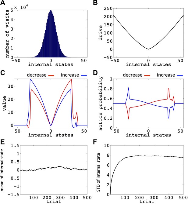
Simulation results replicating Figure 6, with the difference that the initial internal state was zero.
(A) The number of visits at each internal state after 106 trials. (B) The drive function in the one-dimensional homeostatic space (setpoint=0). Value function (C) and choice preferences (D) for state-action pairs after simulating one agent for 106 trials. The mean (E) and standard deviation (F) of the internal state of 105 agents, along 1500 trials.
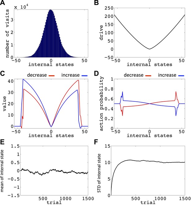
Simulation results replicating Figure 6, with the difference that the initial internal state was zero, and the rate of exploration, β, was 0.03.
(A) The number of visits at each internal state after 106 trials. (B) The drive function in the one-dimensional homeostatic space (setpoint=0). Value function (C) and choice preferences (D) for state-action pairs after simulating one agent for 106 trials. The mean (E) and standard deviation (F) of the internal state of 105 agents, along 1500 trials.
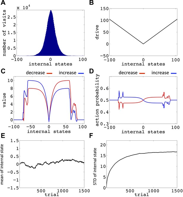
Simulation results replicating Figure 6, with the difference that the initial internal state was zero, and also m = n = 1.
(A) The number of visits at each internal state after 106 trials. (B) The drive function in the one-dimensional homeostatic space (setpoint=0). Value function (C) and choice preferences (D) for state-action pairs after simulating one agent for 106 trials. The mean (E) and standard deviation (F) of the internal state of 105 agents, along 1500 trials.
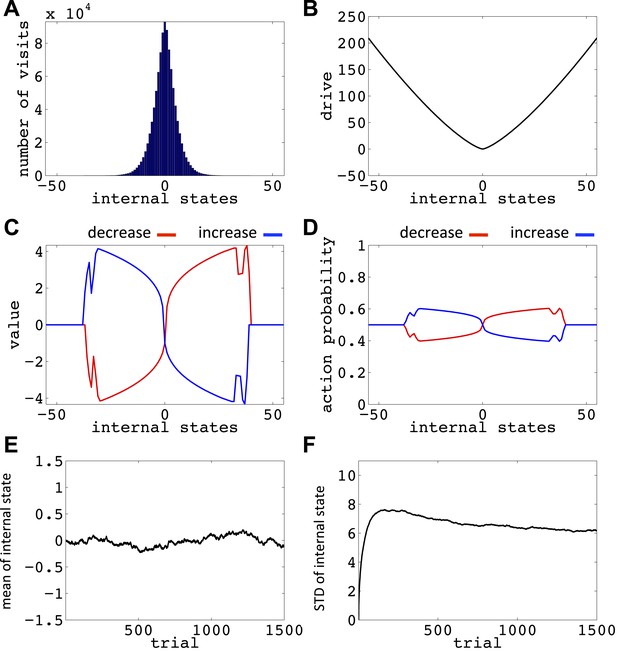
Simulation results replicating Figure 6, with the difference that the initial internal state was zero, and the discount factor, γ, was zero.
(A) The number of visits at each internal state after 106 trials. (B) The drive function in the one-dimensional homeostatic space (setpoint=0). Value function (C) and choice preferences (D) for state-action pairs after simulating one agent for 106 trials. The mean (E) and standard deviation (F) of the internal state of 105 agents, along 1500 trials.
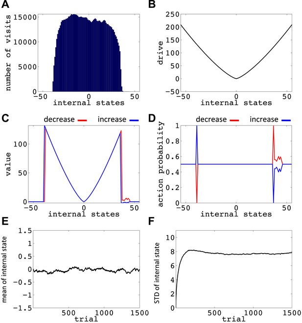
Simulation results replicating Figure 6, with the difference that the initial internal state was zero, and the discount factor, γ, was one (no discounting).
(A) The number of visits at each internal state after 106 trials. (B) The drive function in the one-dimensional homeostatic space (setpoint=0). Value function (C) and choice preferences (D) for state-action pairs after simulating one agent for 106 trials. The mean (E) and standard deviation (F) of the internal state of 105 agents, along 1500 trials.
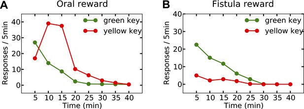
Experimental results (adapted from McFarland, 1969) on learning the reinforcing effect of oral vs. intragastric delivery of water.
Thirsty animals were initially trained to peck at a green key to receive water orally. In the next phase, pecking at the green key had no consequence, while pecking at a novel yellow key resulted in oral delivery of water in one group (A), and intragastric injection of the same amount of water through a fistula in a second group (B). In the first group, responding was rapidly transferred from the green to the yellow key, and then suppressed. In the fistula group, the yellow key was not reinforced.
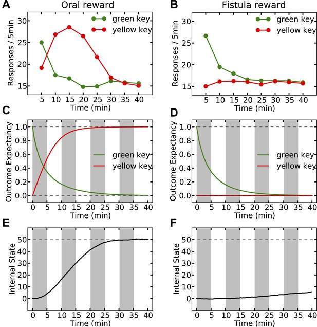
Simulation results replicating the data from McFarland (1969) on learning the reinforcing effect of oral vs. intragastric delivery of water.
As in the experiment, two groups of simulated agents were pre-trained to respond on the green key to receive oral delivery of water. During the test phase, the green key had no consequence, whereas a novel yellow key resulted in oral delivery in one group (A) and intragastric injection in the second group (B). All agents started this phase in a thirsty state (initial internal state = 0; setpoint = 0). In the oral group, responding transferred rapidly from the green to the yellow key and was then suppressed (A) as the internal state approached the setpoint (E). This transfer is due to gradually updating the subjective probability of receiving water outcome upon responding on either key (C). In the fistula group, as the water was not sensed, the outcome expectation converged to zero for both keys (D) and thus, responding was extinguished (B). As a result, the internal state changed only slightly (F).
-
Figure 8—source data 1
Free parameters for the reinforcing vs. satiation simulations.
- https://doi.org/10.7554/eLife.04811.021
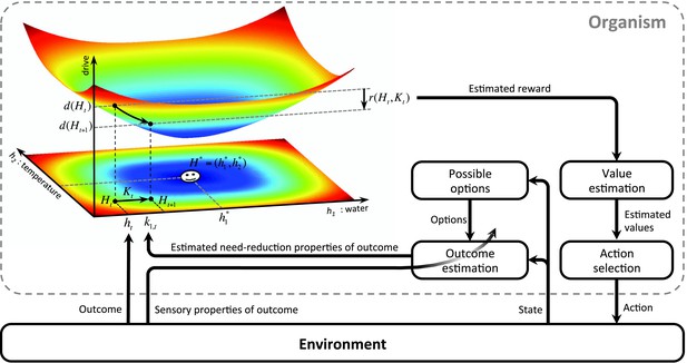
A model-based homeostatic RL system. Upon performing an action in a certain state, the agent receives an outcome, , which results in the internal state to shift from to .
At the same time, sensory properties of the outcome are sensed by the agent. Based on this information, the agent updates the state-action-outcome associations. In fact, the agent learns to predict the sensory properties, , of the outcome that is expected to be received upon performing a certain action. Having learned these associations, the agent can estimate the rewarding value of different options. That is, when the agent is in a certain state, it predicts the outcome , expected to result from each behavioral policy. Based on and the internal state , the agent can approximate the drive-reduction reward.
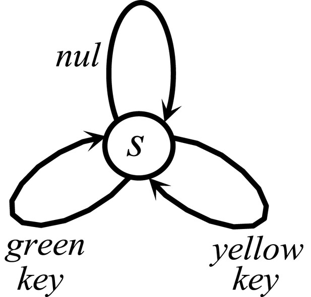
The Markov Decision Process used for simulating the reinforcing vs. satiation effects of water.
At each time point, the agent can choose between doing nothing (nul) or pecking at either the green or the yellow key.
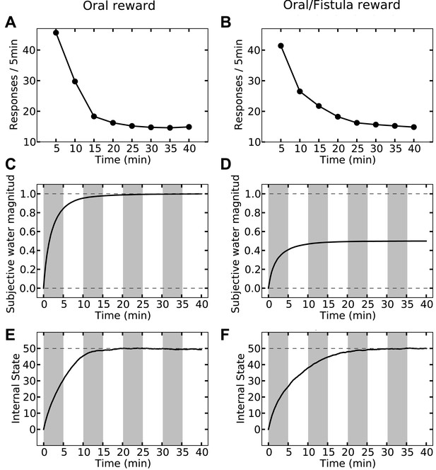
Simulation results of the satiation test.
Left column shows results for the case where water was received only orally. Rate of responding drops rapidly (A) as the internal state approaches the setpoint (E). Also, the agent learns rapidly that upon every key pecking, it receives 1.0 unit of water (C). On the right column, upon every key-peck, 0.5 unit of water is received orally, and 0.5 unit is received via the fistula. As only oral delivery is sensed by the agent, the subjective outcome-magnitude converges to 0.5 (D). As a result, the reinforcing value of key-pecking is less than that of the oral case and thus, the rate of responding is lower (B). This in turn results in slower convergence of the internal state to the setpoint (F). The MDP and the free parameters used for simulation are the same as in Figure 8.
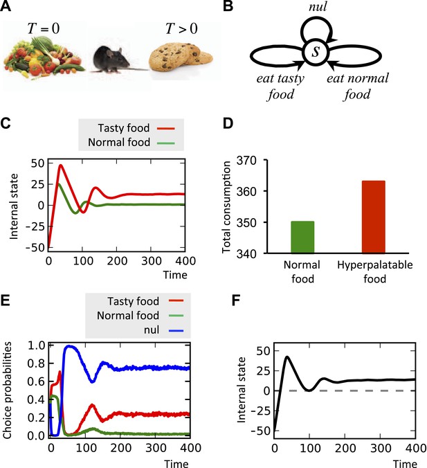
Simulating over-eating of hyperpalatable vs. normal food.
(A) The simulated agent can consume normal (T = 0) or hyperpalatable (T > 0) food. The nutritional content, K, of both foods are equal. In the single-option task (C, D), one group of animals can only choose between normal food and nothing (nul), whereas the other group can choose between hyperpalatable food and nothing. Starting the task in a deprived state (initial internal state=−50), the internal state of the second, but not the first, group converges to a level above the setpoint (C) and the total consumption of food is higher in this group (D). In the multiple-choice task, the agents can choose between normal food, hyperpalatable food, and nothing (B). Results show that the hyperpalatable food is preferred over the normal food (E) and the internal state is defended at a level beyond the setpoint (F). See Figure 10—source data 1 for simulation details.
-
Figure 10—source data 1
Free parameters for the over-eating simulations.
- https://doi.org/10.7554/eLife.04811.026
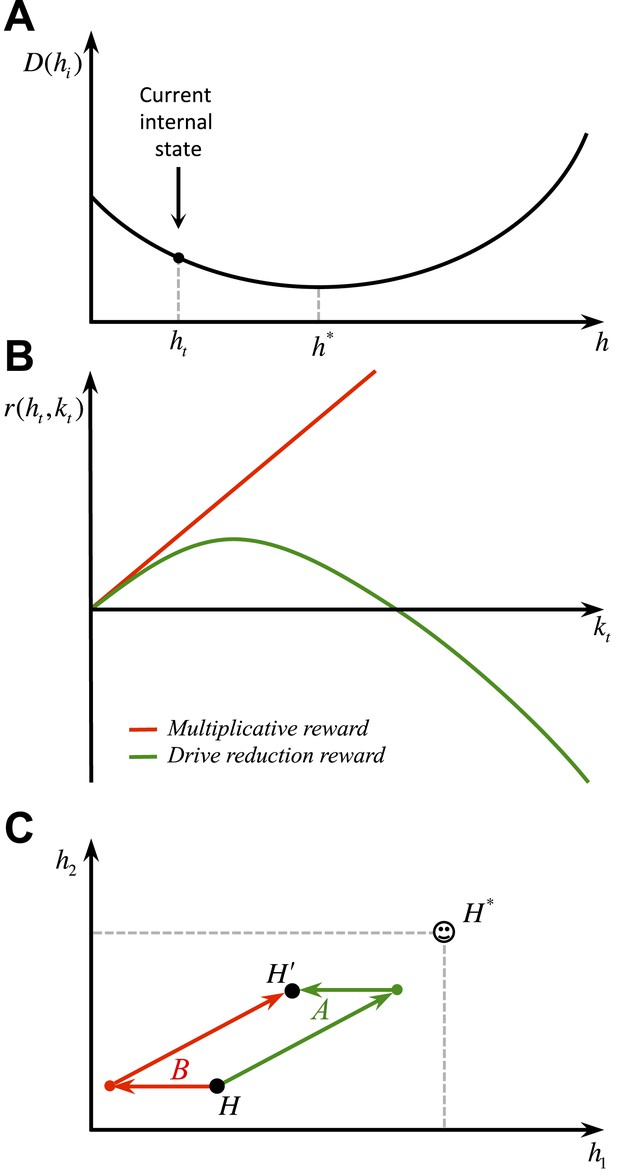
Behavioral predictions of the model.
(A) Differential predictions of the multiplicative (linear) and drive-reduction (non-linear) forms of reward. In our model, assuming that the internal state is at (A), outcomes larger than result in overshooting the setpoint and thus a declining trend of the rewarding value (B). Previous models, however, predict the rewarding value to increase linearly as the outcome increases in magnitude. (C) Our model predicts that when given a choice between two options with equal net effects on the internal state, animals choose the option that first results in reducing the homeostatic deviation and then is followed by an increase in deviation (green), as compared to a reversed-order option (red).
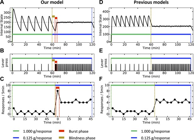
Simulation results, predicting a transitory burst of responding upon reducing the dose of outcome.
Our model (left column) and negative-feedback models (right column) are simulated is a process where responding yields big and small outcomes, during the first and second hours of the experiment, respectively. In our model, the objective is stay as close as possible to the setpoint (A), whereas in previous homeostatic regulation models, the objective is to stay above the setpoint (D). Thus, our model predicts a short-term burst of responding after the dose reduction, followed by regular and escalated response rate (B, C). Classical HR models, however, predict an immediate transition from a steady low to a steady high response rate (E, F). See Figure 12—figure supplements 1 and Figure 12—source data 1 for simulation details.
-
Figure 12—source data 1
Free parameters for the within-session dose-change simulation.
- https://doi.org/10.7554/eLife.04811.029
