Social networks predict gut microbiome composition in wild baboons
Figures
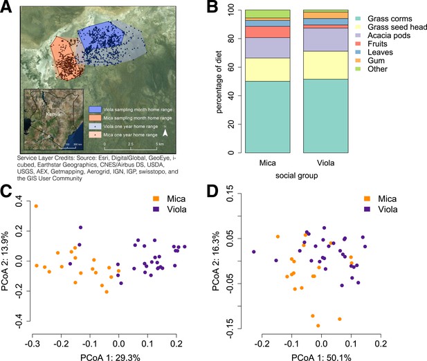
Social group membership predicts microbiome composition.
(A) Group home ranges in the year prior to and during sample collection. (B) Diet composition during sample collection. Only the proportion of fruit consumed significantly differed between groups (p = 0.05; Supplementary file 7). Principal coordinates plots of Bray–Curtis dissimilarity matrices for (C) taxonomic (Supplementary file 2) and (D) KEGG enzyme ortholog composition of individual gut microbiomes (Supplementary file 5). Social group membership explained significant variation in gut microbial composition (PERMANOVA: r2 = 0.186, p < 10−4) as well as gut microbial enzyme ortholog composition (r2 = 0.108, p = 0.003). Relative abundances of common bacterial phyla and KEGG enzyme orthologs are shown in Figure 1—figure supplement 1, 2. A rarefaction analysis of species-level sampling is shown in Figure 1—figure supplement 3. The results of the HUMAnN pipeline are shown in Figure 1—figure supplement 4. A comparison between baboon and human microbiome composition across body sites is shown in Figure 1—figure supplement 5.
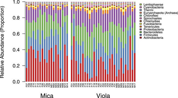
Proportional representation of common phyla in each sample.
The OTU table generated using MetaPhlAn 2.0 was collapsed to the level of the phylum for each sample. Phyla that were not represented at ≥ 1% in at least one of sample are summed and presented as ‘rare phyla.’ Samples from Mica's group are clustered on the left and those from Viola's group on the right.
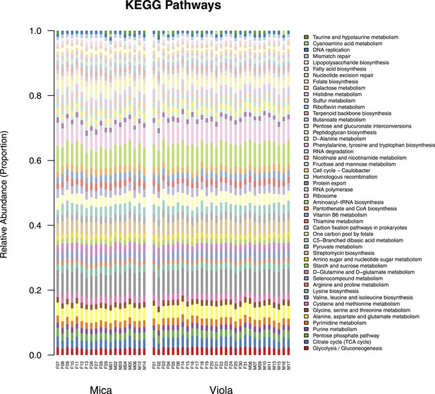
Proportional representation of common KEGG orthologs in each sample, summarized as pathways.
The KEGG pathway abundances generated using HUMAnN were filtered to only include those represented at ≥ 1% in at least one sample and are presented as stacked bar plots. Samples from Mica's group are clustered on the left and those from Viola's group on the right.
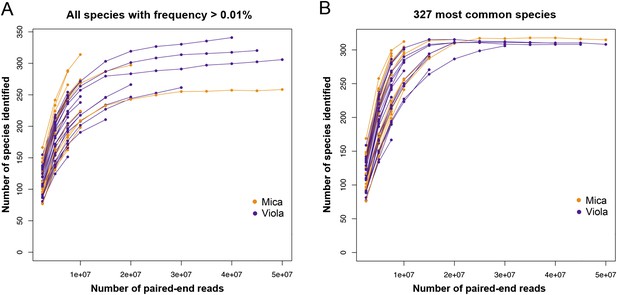
Rarefaction analyzes of shotgun metagenomic data.
Plot (A) shows the number of species found in each sample as a function of the number of paired-end reads down-sampled from the full data set. The number of species reported in each data point corresponds to the average number of species over 10 randomly resampled data sets (restricted to species detected at an abundance >0.01% in the sample, based on the logic that very rare species are more likely to represent assignment errors). In each random re-sampling, we down-sampled the number of reads and re-ran the subsampled sequences through the MetaPhlAn 2.0 pipeline to obtain a count of the number of species represented in each down-sampled data set. Plot (B) depicts a parallel analysis to (A), but limited to the 327 most prevalent species in our data set.
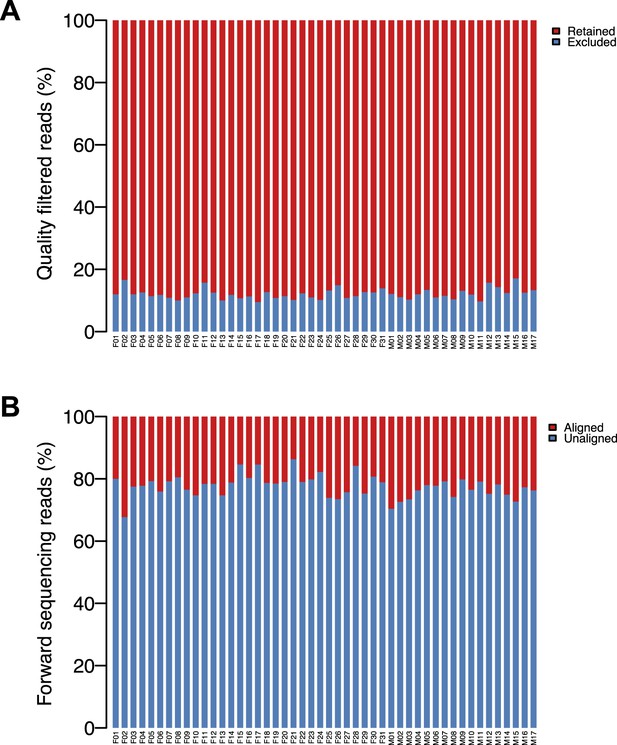
HUMAnN pipeline results.
(A) Percentage of reads retained following quality filtering in usearch, per sample. (B) Percentage of pass-filter reads aligned against an entry in the reduced KEGG database, per sample.
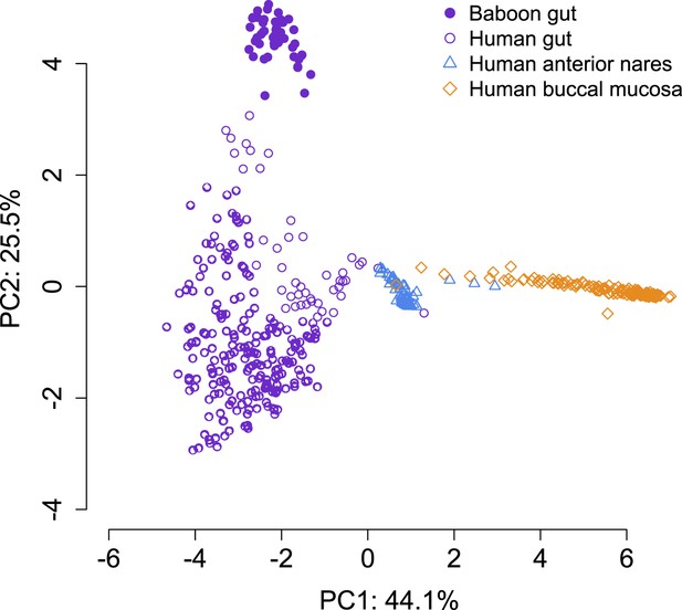
PCA projection of baboon gut microbiome data and Human Microbiome Project data collected from different body sites.
Gut microbiome data from baboons most closely resembles gut microbiome data from humans. The first principal component of the microbiome data separates out data from different body sites; the second principal component separates baboon gut microbiome data from human gut microbiome data.
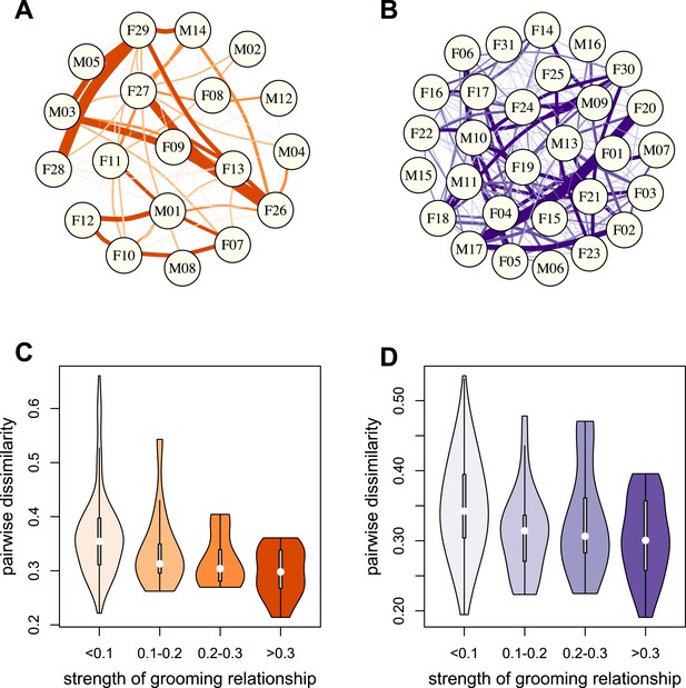
Grooming-based social networks predict microbiome composition.
Social networks based on grooming interactions in the year prior to and including the month of microbiome sampling in (A) Mica's and (B) Viola's social groups. Each circle represents an individual (with the individual's ID listed within the circle). Lines represent grooming interactions between individuals, and heavier lines reflect stronger grooming relationships. (C and D) Violin plots depicting the relationships between pairwise grooming bond strength vs pairwise Bray–Curtis dissimilarity in taxonomic composition in Mica's and Viola's groups, respectively. White dots represent median values and grey rectangles represent the first and third quartiles of the data. Rotated kernel density plots representing the underlying data are shown on each side. Stronger bonds predict more similar gut microbiotas in both groups (Mica's group: Mantel test r = −0.257, p = 3.0 × 10⁻⁴; Viola's group: r = −0.173, p = 8.0 × 10⁻⁴). Parallel results based on de novo assembly are shown in Figure 2—figure supplement 1.
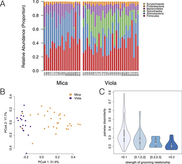
Evidence for social structuring of the gut microbiome based on de novo assembly.
Estimating gut microbiome taxonomic composition by comparison to de novo bacterial genome assemblies also produces congruent evidence for social structuring. (A) Proportional representation of common phyla in each sample, grouping phyla not present at >1% in at least one sample together are ‘rare phyla’. (B) Principal coordinates projection for individuals from Mica's group and Viola's group separates samples by social group along the first axis. (C) Strength of pairwise grooming relationships, and thus within group social structure, explains levels of similarity and dissimilarity in gut microbiome taxonomic composition. Data are shown for Mica's group.
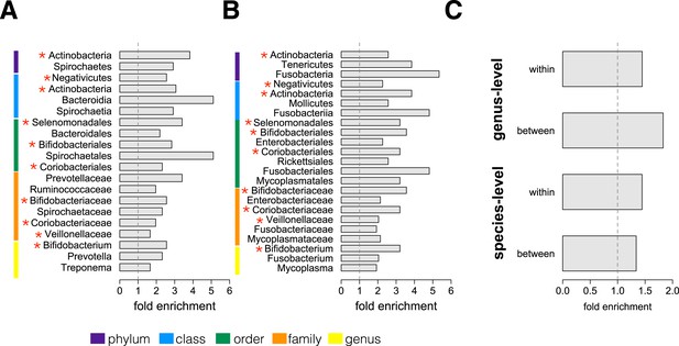
Socially structured species are taxonomically and phenotypically nonrandom.
Bacterial taxonomic groups significantly enriched (10% FDR) for socially structured species (A) between social groups and (B) within the grooming network for Viola's group (Supplementary file 8). Vertical dashed lines depict a fold enrichment of 1, representing the background level of taxon abundance in the data set. Red asterisks denote taxonomic groups identified as significantly enriched at both levels of analysis. (C) Significant enrichment of anaerobic, non-spore-forming bacterial taxa, both between and within groups, at both species and genus levels (socially structured species between groups, species level traits: p = 0.017; socially structured species within group, species level traits: p = 0.067; socially structured species between groups, genus level traits: p = 0.036; socially structured species within group, genus level traits: p = 0.040). See Figure 3—figure supplements 1, 2 for a comparison of the enrichment of p-values in our data set vs an empirical null distribution.
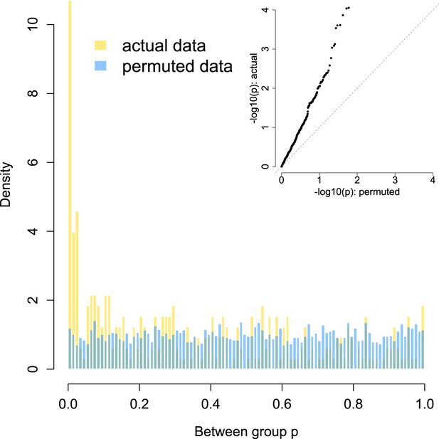
Enrichment of low p-values in the data vs an empirical null: between group analyses.
To confirm that our modeling approach (quantile normalization of species relative abundances, followed by mixed effects modeling in GEMMA) did not bias us towards detecting false positives, we compared the signal in our true data set against an empirically derived null. The histogram distribution of p-values for the true data (gold) is plotted against the distribution of p-values from 10 permutations (blue). In each permutation, group membership was scrambled across the data set while keeping the modeling approach, kinship structure, and all other covariates constant. The inset shows a quantile–quantile plot of the same data, with clear enrichment of differentially abundant species in the actual data vs the empirical null. No differentially abundant species are detected at a 10% FDR in the permuted data sets, while 64 are discovered in the true data set.
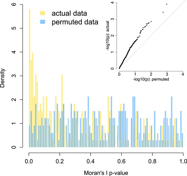
Enrichment of low p-values in the data vs an empirical null: within group network analysis.
To confirm that our modeling approach (Moran's I statistic within Viola's group) did not bias us towards detecting false positives, we compared the signal in our true data set against an empirically derived null. The histogram distribution of p-values for the true data (gold) is plotted against the distribution of p-values from 10 permutations (blue). In each permutation, species abundance was scrambled across group members while keeping the modeling approach and social network structure constant. The inset shows a quantile–quantile plot of the same data, with clear enrichment of socially structured species in the actual data vs the empirical null. No socially structured species are detected at a 10% FDR in the permuted data sets, while 51 are discovered in the true data set.
Additional files
-
Supplementary file 1
Table listing all subject and sample characteristics.
- https://doi.org/10.7554/eLife.05224.014
-
Supplementary file 2
Table listing the relative abundance of microbial species in each sample inferred via MetaPhlAn 2.0.
- https://doi.org/10.7554/eLife.05224.015
-
Supplementary file 3
Table listing species richness and alpha diversity for each sample based on taxonomic profiling using MetaPhlAn 2.0 and de novo contig assembly.
- https://doi.org/10.7554/eLife.05224.016
-
Supplementary file 4
Table listing species proportional abundance for each sample based on de novo contig assembly.
- https://doi.org/10.7554/eLife.05224.017
-
Supplementary file 5
Table listing the relative abundance of enzyme gene orthologs in each sample.
- https://doi.org/10.7554/eLife.05224.018
-
Supplementary file 6
Table listing the proportional representation of common phyla in each sample. Taxonomic abundances were inferred for all samples using MetaPhlAn 2.0.
- https://doi.org/10.7554/eLife.05224.019
-
Supplementary file 7
Table listing the dietary composition during the microbiome sample collection period.
- https://doi.org/10.7554/eLife.05224.020
-
Supplementary file 8
Table listing statistical evidence for social structuring for the 327 most common bacterial species (prevalence >50% across 48 samples). Between group analyses were based on the linear mixed modeling approach implemented in the program GEMMA; q-values reflect a false discovery rate of 10%. Within-network analyses were based on Moran's I, as implemented in the function Moran.I in the R package ape; q-values reflect a false discovery rate of 10%.
- https://doi.org/10.7554/eLife.05224.021


