Distinct cortical codes and temporal dynamics for conscious and unconscious percepts
- Institut National de la Santé et de la Recherche Médicale, France
- Institut d'Imagerie Biomédicale, France
- Ben-Gurion University of the Negev, Israel
- Aalto University School of Science, Finland
- University of Oxford, United Kingdom
- Collège de France, France
- University of Paris-Sud, France
Figures
Figure 1
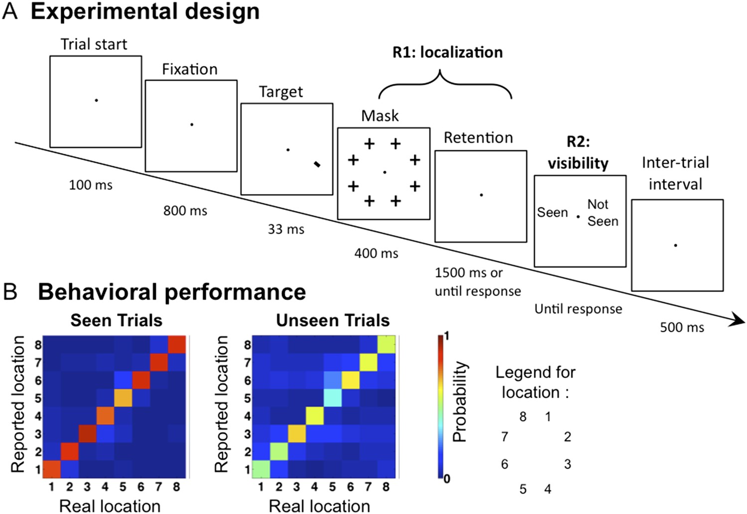
Experimental design and behavioral results.
(A). Sequence of events presented on a trial. Subjects attempted to localize a brief target, which could appear at one of eight locations. Mask contrast was adjusted to ensure ∼50% of unseen trials. On 1/9 of trials, the target slide was replaced by a blank slide (target-absent trial). (B) Behavioral confusion matrices describing the distribution of responses for each spatial location when target was seen (left matrix) or unseen (right matrix). A strong diagonal on unseen trials indicates blindsight.
Figure 2 with 4 supplements
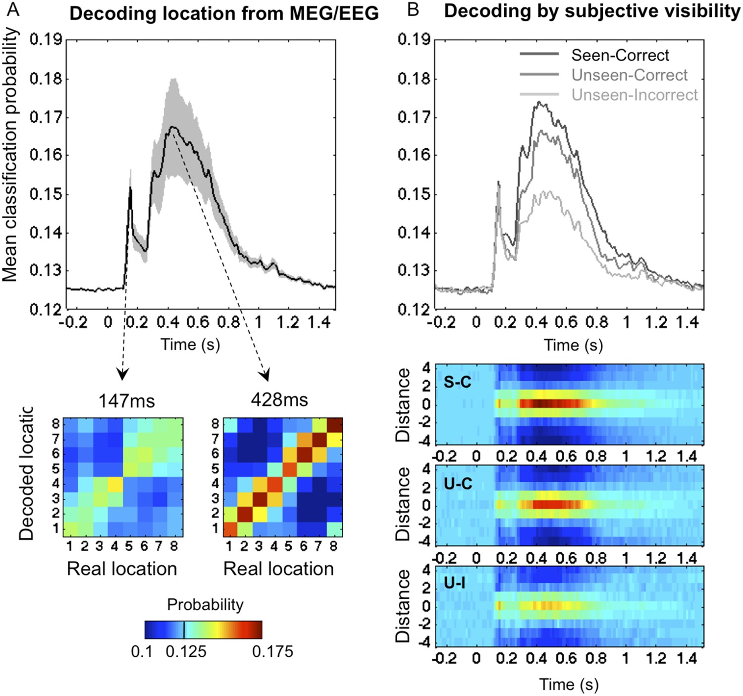
Time course of location information.
(A). Average posterior probability of a correct classification of target location, as a function of time. Chance = 12.5% (1/8). Decoding confusion matrices are shown at the two decoding peaks. (B) Same data sorted as a function of subjective visibility (seen/unseen) and objective localization performance (correct/incorrect). The lower part shows the time course of average classifier probability as a function of distance between the decoded and actual target location.
Figure 2—figure supplement 1
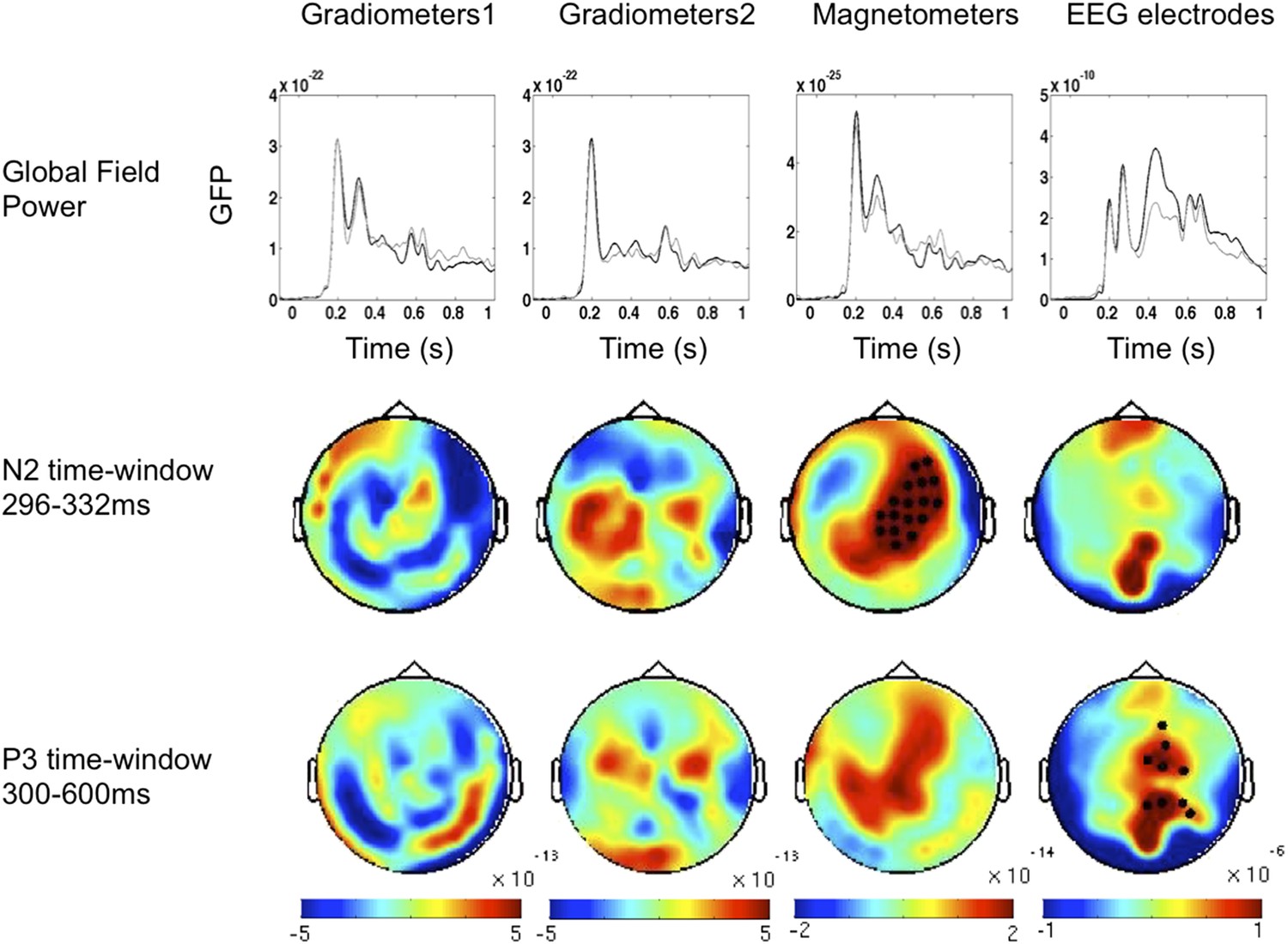
Event-Related Fields and potentials for ‘Seen–Correct’ vs ‘Unseen–Correct’.
ERF and ERP components time windows were determined according to the global field power (upper panel). Two time windows were chosen; on each time window, cluster analysis was performed. In the 296–332 ms time window, Magnetometers showed a significant cluster (p = 0.025). EEG electrodes exhibited a significant cluster on the 300–600 ms time window p = 0.02.
Figure 2—figure supplement 2

Event-Related Fields and potentials for ‘UnSeen–Correct’ vs ‘Unseen–InCorrect’.
ERF and ERP components time windows were determined according to the global field power (upper panel). Two time windows were chosen; on each time window, cluster analysis was performed. No significant differences were found.
Figure 2—figure supplement 3
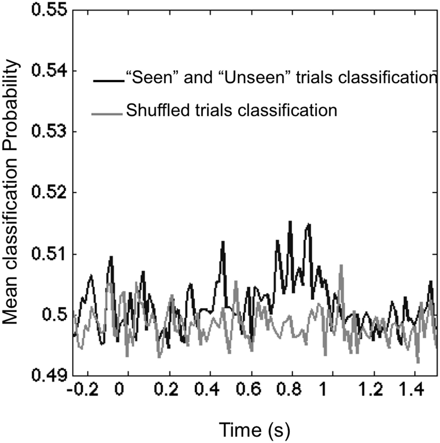
Classifying visibility.
The black line portrays the mean classification probability of classifier trained to classify ‘Seen–Correct’ and ‘Unseen–Correct’. The lighter line portrays classifier trained on the dataset with shuffled classes. In the 270–800 ms time window, mean classification probability (0.503 ± 0.001) was slightly higher than chance (0.5) t(11) = 2.45, p = 0.03. Shuffled trials classification probability (0.498 ± 0.001) did not differ from chance t(11) = 2.11, p = 0.057.
Figure 2—figure supplement 4
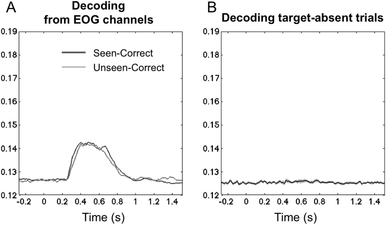
Controls for eye movements and motor-based decoding.
(A) Average posterior probability of a correct classification of target location, across time, separately for ‘Seen–Correct’ and ‘Unseen–Correct’ trials, for classifiers trained on EOG channels only. Eye-based decoding is much lower than with the full set of sensors and, crucially, does not differentiate seen and unseen trials. Classification rose above chance 256 ms post stimuli and went back to chance 1000 ms post stimuli. Importantly, within this time frame, classification for ‘Seen–Correct’ (0.135 ± 0.001) and ‘Unseen–Correct’ (0.134 ± 0.001) did not differ t(11) < 1. (B) Average posterior probability of a correct classification of the manual response on target-absent trials, across time. Classifiers were trained on target's location in valid trials and tested on responses in absent trials. A flat curve indicates that target location decoding reported in the results section did not rely on motor preparation and execution information.
Figure 3
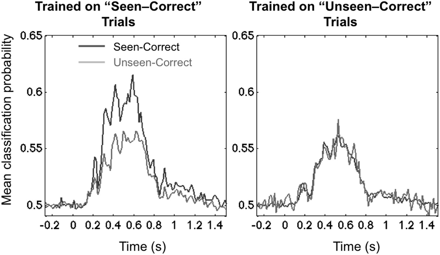
Asymmetrical cross-condition generalization.
A classifier trained in one condition and then tested on new data either from the same condition or the other condition (e.g. trained on ‘Seen–Correct’ trials and tested on new ‘Seen–Correct’ trials and ‘Unseen–Correct’ trials). To equalize the number of trials, the classifier was trained to discriminate left- vs right-hemifield targets, hence chance = 50%.
Figure 4 with 1 supplement
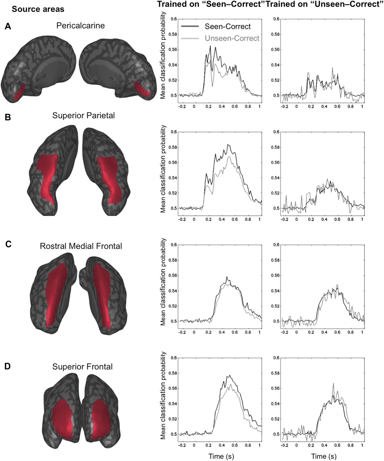
Source-based decoding and cross-condition generalization.
Classifiers were trained as in Figure 3, but using a restricted subset of cortical sources: pericalcarine (A), superior parietal (B), rostro-medial frontal (C), or superior frontal (D). Note, how asymmetrical cross-condition generalization (right columns, same format as Figure 3) successively arises in visual cortex, then superior parietal, and superior frontal regions.
Figure 4—figure supplement 1
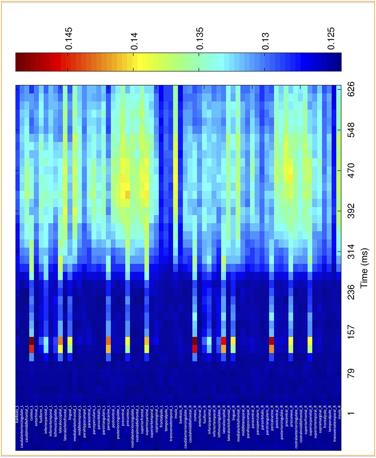
Time course of location information for the different cortical sources.
Average posterior probability of a correct classification of target location, as a function of time for in 68 regions of interest. Chance = 12.5% (1/8).
Figure 5 with 3 supplements
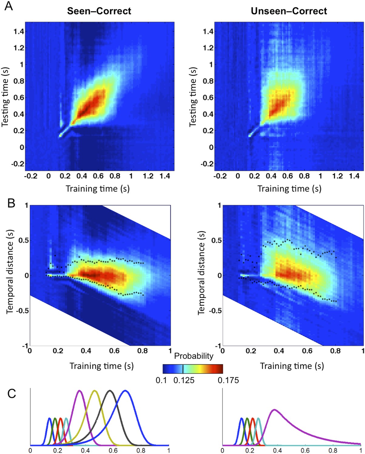
Generalization of location decoding over time.
8-location classifiers trained at a specific time were then tested on data from all other time points. (A) Average classification probability as a function of testing time for each training time (the diagonal, where testing time = training time, gives the curve for classical decoder performance over time). (B) Same information plotted as a function of temporal distance from training time (positive or negative), with asterisks indicating the Classification Endurance (CE) measure. (C) Tentative model of a sequence of brain activations, which could yield the observed generalization matrices.
Figure 5—figure supplement 1

Analysis of variance (ANOVA) on Classification Endurance (CE).
The table gives the statistics and significance values for the main effects of Visibility (Seen–Correct vs Unseen–Correct), Direction of generalization (forward, backward), and Timeframe (5 levels), as well as their interactions.
Figure 5—figure supplement 2
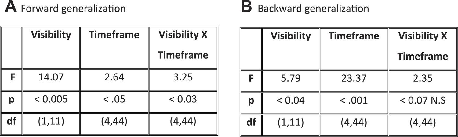
ANOVAs on CE with factors of Visibility (Seen–Correct vs Unseen–Correct) and Timeframe (5 levels), separately for forward and backward generalization.
(A) Forward generalization (B) Backward generalization.
Figure 5—figure supplement 3
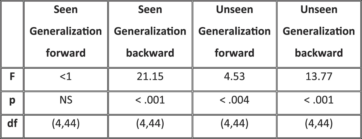
Significance Values of the Effect of Timeframe (5 levels) for forward and backward generalization in Seen and unseen trials.
https://doi.org/10.7554/eLife.05652.015Download links
A two-part list of links to download the article, or parts of the article, in various formats.
Downloads (link to download the article as PDF)
Open citations (links to open the citations from this article in various online reference manager services)
Cite this article (links to download the citations from this article in formats compatible with various reference manager tools)
Distinct cortical codes and temporal dynamics for conscious and unconscious percepts
eLife 4:e05652.
https://doi.org/10.7554/eLife.05652


