Limits on information transduction through amplitude and frequency regulation of transcription factor activity
- Howard Hughes Medical Institute, Harvard University, United States
- Harvard University, United States
Figures
Figure 1
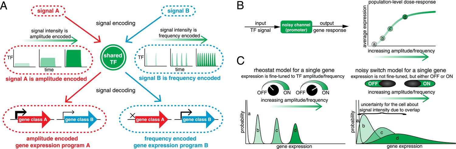
Encoding and transmitting signal identity and intensity information in the dynamics of a single transcription factor (TF).
(A) Different signals (e.g., stress or ligand exposure) can be encoded in the dynamics of a single TF. Signal identity is encoded in the type of TF dynamics: a sustained pulse (signal A) or nuclear pulsing (signal B). Signal intensity (e.g., ligand concentration) is encoded in the amplitude for signal A, but in the frequency for signal B. Different dynamical patterns of TF activation can activate distinct, but specific, downstream gene expression programs. (B) Applying an information theoretic framework to cell signaling, a gene promoter can be considered a channel. A graded population-level dose–response belies the complexity of the single-cell response: it shows the mean expression at points a, b, c, and d, but not the width or variance of their distributions. (C) Two extreme models. In the ‘rheostat model’, signal intensity information encoded in the frequency or amplitude of a TF leads to non-overlapping gene expression distributions (a, b, c, and d). Thus, by reading the gene expression output the cell can accurately determine the input signal intensity and high information transmission is achieved. Conversely, in the ‘noisy switch model’, as a consequence of overlapping gene expression distributions (a, b, c, and d) information about signal intensity is permanently lost: the cell can distinguish ON/OFF (signal identity), but the expression of a target gene cannot be fine-tuned to the stress intensity.
Figure 2 with 2 supplements

Information transduction by promoters with respect to amplitude and frequency modulation.
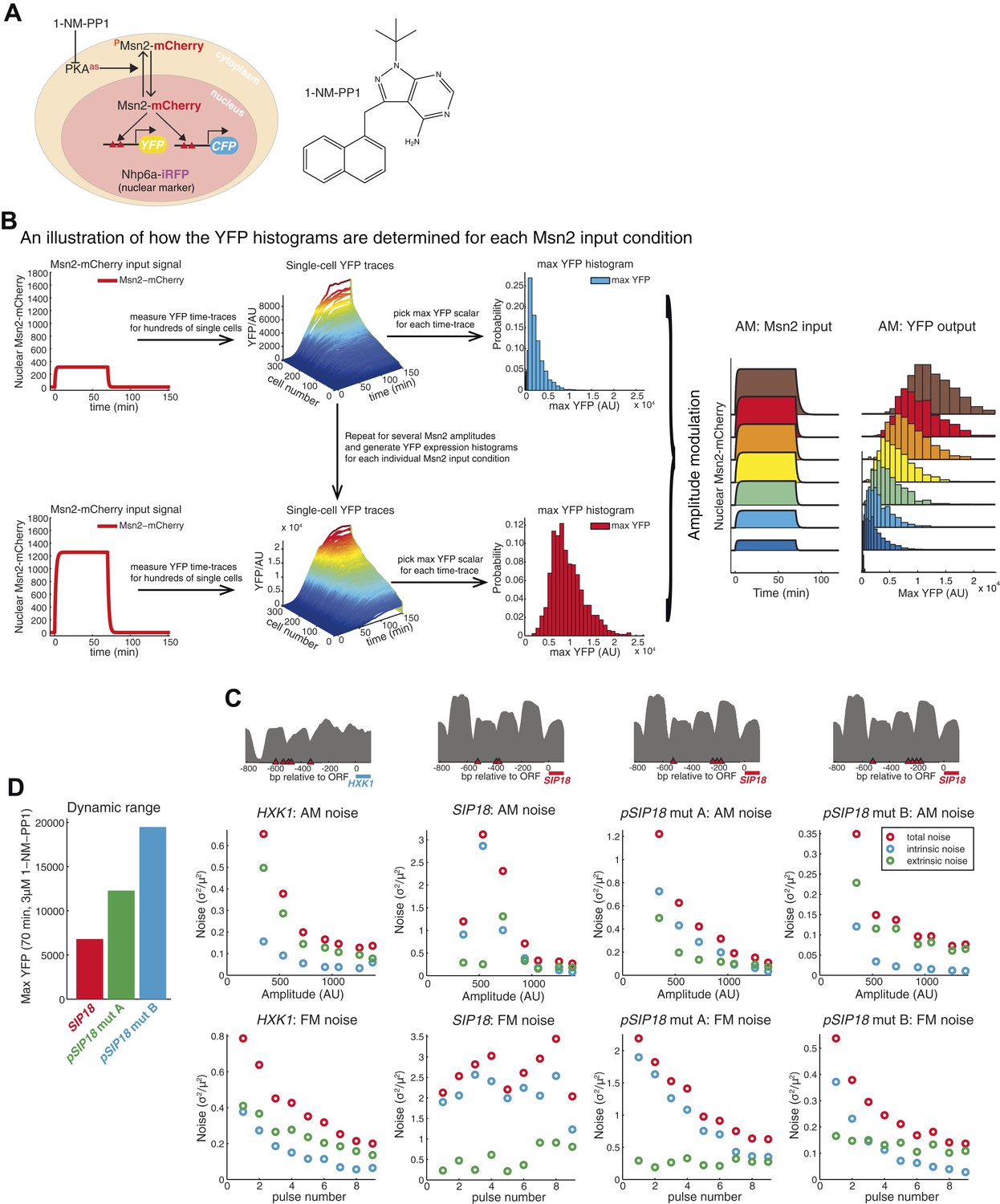
(A) Cells containing either the hxk1::YFP or sip18::YFP reporter were exposed to either no activation or a 70-min pulse of seven increasing amplitudes from ca. 25% (100 nM 1-NM-PP1) to 100% (3 μM 1-NM-PP1) of maximal Msn2-mCherry nuclear localization and single-cell gene expression monitored. For each single-cell time-trace, YFP concentration is converted to a scalar by taking the maximal YFP value after smoothing. For each Msn2-mCherry input (a fit to the raw data is shown on the left (AM: Msn2 input)), the gene expression distribution is plotted as a histogram of the same color on the right for HXK1 and SIP18. The population-averaged dose–response (top) is obtained by calculating the YFP histogram mean for each Msn2 input condition. (B) Cells containing either the hxk1::YFP or sip18::YFP reporter were exposed to either no activation or from one to nine 5-min pulses of Msn2-mCherry nuclear localization (ca. 75% of maximal nuclear Msn2-mCherry, 690 nM 1-NM-PP1) at increasing frequency. All calculations were performed as in (A). (C) Cells containing either the pSIP18 mut A::YFP reporter or the pSIP18 mut B::YFP reporter were exposed to amplitude modulation (AM) as in (A). (D) Cells containing either the pSIP18 mut A::YFP reporter or the pSIP18 mut B::YFP reporter were exposed to frequency modulation (FM) as in (B). Maximal mutual information, I, and its error are calculated as described in Supplementary file 2. Full details on data processing are given in ‘Materials and Methods’. Each plot of an Msn2 input pulse and YFP expression is based on data from ca. 1000 cells from at least three replicates. All raw single-cell time-lapse microscopy source data for HXK1 (15,259 cells), SIP18 (21,242 cells), pSIP18 mut A (18,203 cells), and pSIP18 mut B (17,655 cells) for this Figure are available online as Supplementary file 1 and in (Hansen and O'Shea, 2015).
Figure 2—Figure supplement 1
How time-lapse data are converted to histograms and promoter maps and noise data.
(A) Overview of strains. To visualize and quantify the subcellular localization of Msn2 it was C-terminally tagged with the red fluorescent protein mCherry. A nuclear protein, NHP6a, was C-terminally tagged with iRFP, an infrared fluorescent protein (Filonov et al., 2011; Hansen and O'Shea, 2013), to visualize the nucleus for segmentation purposes. All three catalytic subunits of Protein Kinase A (PKA) were mutated to contain an analogue-sensitive M→G mutation (TPK1M164G TPK2M147G TPK3M165G). These mutations render all three PKA subunits sensitive to the small molecule 1-NM-PP1 (Bishop et al., 2000; Hao and O'Shea, 2012; Zaman et al., 2009). Thus, when 1-NM-PP1 is added, PKA is inhibited, Msn2-mCherry is no longer phosphorylated by PKA, Msn2-mCherry therefore gets dephosphorylated, and translocates into the nucleus where it can bind to and activate target genes. To visualize gene expression, the ORFs of target genes were replaced with YFP (mCitrineV163A) and CFP (SCFP3A) on homologues chromosomes in diploid cells, as it has been described previously (Hansen et al., 2015; Hansen and O'Shea, 2013; Kremers et al., 2006). The inhibitor, 1-NM-PP1 is shown on the right and its synthesis has been described previously (Hansen and O'Shea, 2013). (B) An illustration of how the YFP histograms are obtained for each condition. For a specific amplitude or frequency, the response of ∼1000 cells is measured (only ∼300 cells shown here for ease of visualization). For each single cell time-trace, a moving average smoothing filter is applied to remove any technical noise and the maximal YFP value is determined after the trace has reached a plateau. This is repeated for all single cells and a YFP histogram is generated by binning. The procedure is then repeated for all the Msn2 conditions (e.g., the no input and all the AM conditions) to generate a full single-cell dose–response (right). These data are then used to calculate the maximal mutual information with respect to amplitude modulation, IAM. (C) Promoter nucleosome occupancy maps. The upstream promoter region (−800 to 0 bp from ATG site) is shown for each promoter. Msn2 binding sites (STRE 5′-CCCCT-3′) are shown in red triangles and nucleosome occupancy data (grey) are from (Hansen and O'Shea, 2013). The SIP18 promoter has three Msn2 binding sites. The most upstream site is seemingly non-functional—removing it does not affect gene induction. The two sites (close to −400 bp) are required—removing these two sites abolishes gene induction. pSIP18 mut A and mut B have three and four new binding sites, respectively, in between the two nucleosomes close to the transcription start site. (D) Dynamic range and noise. Removing the two WT Msn2 binding sites and replacing them with three or four binding sites, respectively, substantially increases the dynamic range (defined as the response to a 70 min pulse at 3 μM 1-NM-PP1). How the total (red), intrinsic (blue) and extrinsic (green) noise scales with the Msn2 amplitude (for a 70 min pulse; top) or the frequency (at 690 nM 1-NM-PP1; bottom) for all four promoters is shown. The y-axis scale is different in each case.
Figure 2—Figure supplement 2

Data processing and control of measurement noise.
(A) Data processing illustration. Controlling measurement noise is important, because high measurement noise will cause measurements of mutual information to be underestimates. To minimize effects of measurement noise coming from, for example, improper focusing by the microscope, autofluorescence and camera noise, slight errors in cell segmentation and other sources, multiple YFP measurements are made. For each single cell, the YFP level is measured 64 times at 2.5 min time resolution. In general, measurement noise is modest at very low YFP expression—in part due to cellular autofluorescence—but negligible at high YFP expression. As an example of very low YFP expression, a single cell time-trace is shown on the left (SIP18, 70 min, 100 nM 1-NM-PP1). By smoothing the raw YFP data (black circles), an accurate estimation of the YFP level can be obtained (red line). As an example of very high YFP expression, a raw and smoothed single cell time-trace is shown on the right (mut B, 70 min, 3 μM 1-NM-PP1). (B) Example of raw data at very low YFP expression (SIP18, 70 min, 100 nM 1-NM-PP1). Raw YFP time-traces of 100 randomly chosen single cells are shown on the left and the same YFP time-traces, after smoothing as illustrated in (A), are shown on the right. Although the raw YFP data suffer from modest measurement noise, the actual YFP level can be accurately estimated by smoothing. (C) Example of raw data at low YFP expression (mut A, 70 min, 100 nM 1-NM-PP1). Raw YFP time-traces of 100 randomly chosen single cells are shown on the left and the same YFP time-traces, after smoothing as illustrated in (A), are shown on the right. (D) Example of raw data at high YFP expression (mut B, 70 min, 3 μM 1-NM-PP1). Raw YFP time-traces of 100 randomly chosen single cells are shown on the left and the same YFP time-traces, after smoothing as illustrated in (A), are shown on the right. Furthermore, all raw single-cell time-trace data for HXK1 (15,259 cells), SIP18 (21,242 cells), pSIP18 mut A (18,203 cells), pSIP18 mut B (17,655 cells), 1× reporter diploid (21,236 cells), and 2× reporter diploid (19,222 cells) are available as Supplementary file 1 and in (Hansen and O'Shea, 2015).
Figure 3 with 1 supplement
An algorithm for estimating intrinsic mutual information.
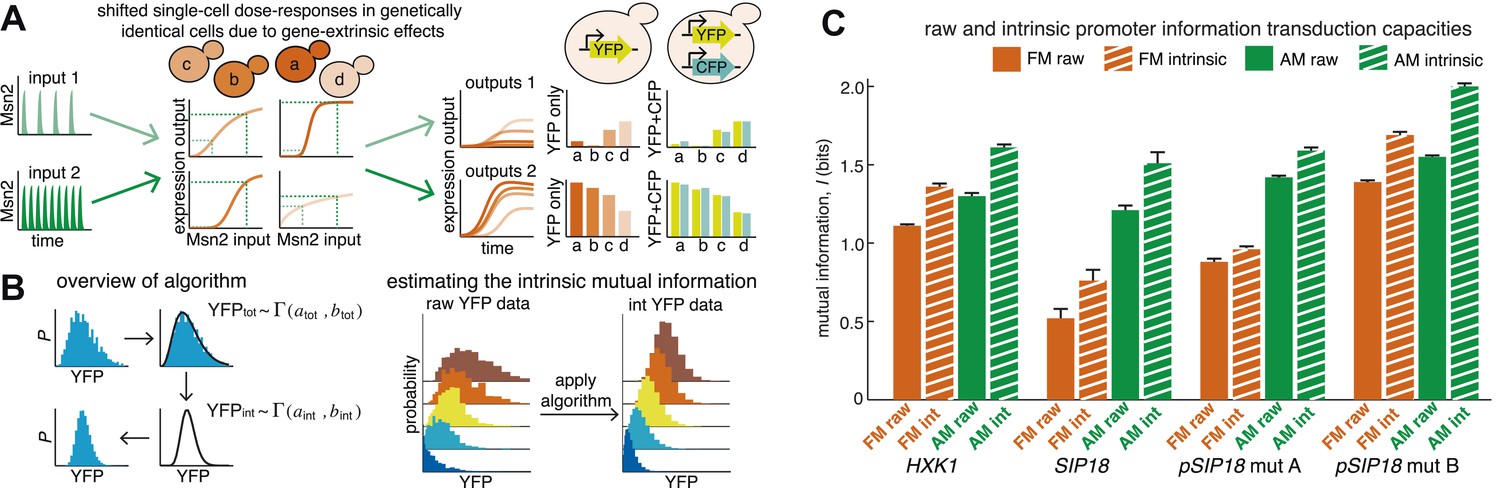
(A) Genetically identical cells can have shifted single-cell dose-responses due to gene-extrinsic effects, such as variation in Msn2 abundance and cell cycle phase. Measuring the response of a single reporter (YFP) therefore underestimates mutual information. By introducing an additional reporter (CFP), we can distinguish extrinsic noise such as a shifted dose–response since this affects both CFP and YFP equally, from true intrinsic stochasticity. (B) Overview of algorithm. By fitting a gamma distribution to the raw YFP data, calculating the CFP/YFP covariance and filtering this component out of the total variance, an intrinsic YFP distribution can be estimated (left). By repeating this for each dose–response distribution, intrinsic mutual information can be estimated (right). Full details on the algorithm are given in Supplementary file 2. (C) By applying the algorithm to the data from Figure 2 (solid bars), we can estimate intrinsic mutual information (hatched bars).
Figure 3—Figure supplement 1
Input noise and variability in Msn2 abundance.
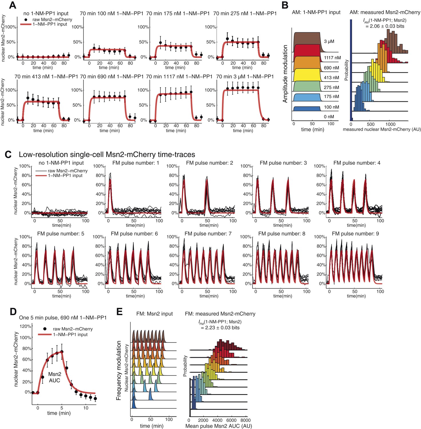
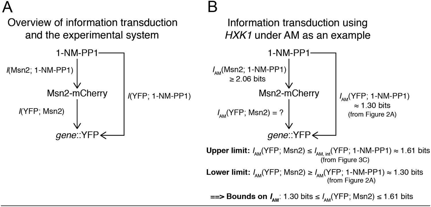
(A) Variability in Msn2 abundance. One source of noise in our system is non-genetic cell-to-cell variability in Msn2 abundance. Msn2 is a low-abundance protein: there are only a few hundred molecules in each cell (Ghaemmaghami et al., 2003). Therefore, precisely measuring Msn2 abundance is challenging. Furthermore, the nucleus moves in and out of focus during time-lapse acquisition. To estimate the variation in Msn2 abundance, cells (pSIP18 mut B) were grown in the microfluidic device and exposed to a 70-min pulse of either 0, 100 nM, 175 nM, 275 nM, 413 nM, 690 nM, 1117 nM or 3 μM 1-NM-PP1. Msn2-mCherry nuclear localization was measured using a 5-frame z-stack series of 0, ±1.2 μm, ± 2.4 μm above and below the focal plane using a 500 ms exposure time and imaging every 10 min. Msn2-mCherry fluorescence was corrected for photobleaching. We collected two frames before and after 1-NM-PP1 exposure to calculate the baseline level of Msn2 before 1-NM-PP1 treatment. In (A), we show the mean and standard deviation for each timepoint for each concentration. (B) To calculate mutual information between 1-NM-PP1 input and Msn2-mCherry dynamics, we use the data from (A) and calculate IAM(1-NM-PP1; Msn2) = 2.06 ± 0.03 bits. We quantify Msn2-mCherry localization in absolute units as the mean nuclear Msn2 level across the seven measurements while Msn2 is nuclear—this also corresponds to the total time-integrated nuclear level of Msn2 (Msn2 ‘Area Under the Curve’ or AUC). In total, we measured 2996 single cells. Using Msn2 variability in response to 3 μM 1-NM-PP1, we estimate the cell-to-cell variability of Msn2 to be CV∼15%. However, given measurement noise we stress that CV∼15% and I∼2.06 bits are likely over- and underestimates, respectively. Note that Msn2 is a low abundance protein (Ghaemmaghami et al., 2003). Previous proteomic studies showed that essentially no yeast proteins have CV<10% (Newman et al., 2006). Therefore, Msn2 is among the least variable low abundance proteins in yeast. (C) This figure is plotted using data from Figure 2 for HXK1 (Hansen and O'Shea, 2015). In red is shown the input and in black is shown traces from 10 representative single cells. We did not do a finely spaced z-stack series for this experiment, which is necessary to accurately quantify the concentration of Msn2 in the nucleus—this causes too much photobleaching to be compatible with imaging at reasonable temporal resolution (2.5 min here). Nonetheless, as can be seen, the black traces faithfully track the input with limited noise. For each cell plotted above, we also measured hxk1::CFP and hxk1::YFP gene expression. (D) To accurately quantify Msn2-mCherry dynamics during FM input, we acquired a finely spaced z-stack series at high time-resolution (1 min). This causes too high photobleaching to be compatible with sustained time-lapse imaging. Therefore, we are only able to collect data at this resolution for a single 5-min pulse. The mean (black dots) and standard deviation (error bars) for 132 single cells (pSIP18 mut B) are shown. As can be seen, Msn2-mCherry accurately tracks the microfluidic 1-NM-PP1 input with limited noise also during FM input. In a population of cells, Msn2 translocates to the nucleus in every single cell during 1-NM-PP1 exposure. (F) To calculate mutual information between 1-NM-PP1 input and Msn2-mCherry dynamics, we use the data from (D) and estimate IFM(1-NM-PP1; Msn2) = 2.23 ± 0.03 bits. Given measurement noise, this is likely an underestimate. We quantify Msn2-mCherry localization in absolute units as the total nuclear Msn2 level across the ten measurements while Msn2 is nuclear (five during the pulse, five after the pulse)—this also corresponds to the total time-integrated nuclear level of Msn2 (Msn2 ‘Area Under the Curve’ or AUC). With data from (D), we measure the distribution of cell-to-cell variability for a single 5-min pulse. To calculate IFM, we then extrapolate by multiplying the AUC probability distribution by the pulse number of each experiment since Msn2 tracks the 1-NM-PP1 input as faithfully for the first pulse as for the subsequent pulses. Ideally, one would measure the Msn2 AUC at 1-min time resolution and with finely spaced z-stacks throughout the entire time-lapse experiment, but this is not technically possible due to photobleaching.
Figure 4 with 2 supplements
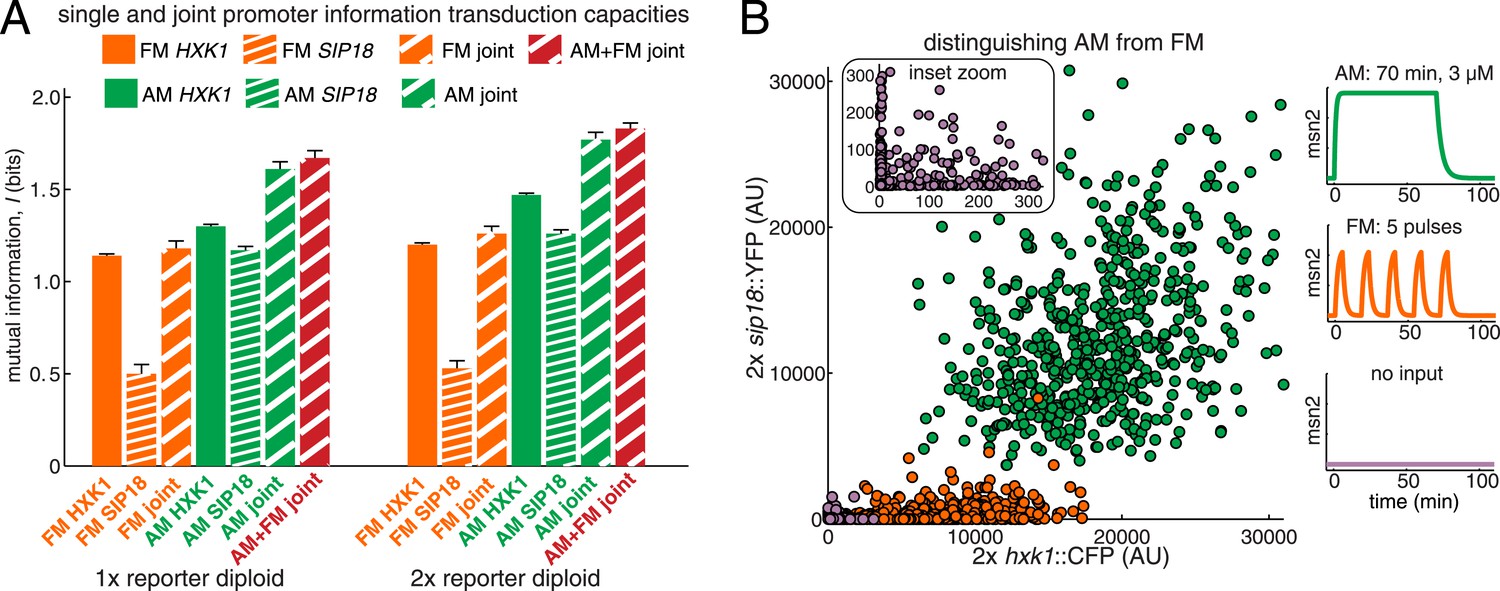
Integrating the response of more than one gene improves information transmission.
(A) The AM and FM experiments (Figure 2) were repeated for diploid strains containing either one copy (1×) of the hxk1::CFP and sip18::YFP reporters or two copies (2×) of the hxk1::CFP and sip18::YFP reporters and individual and joint mutual information determined (full details on calculations are given in Supplementary file 2). (B) 2× sip18::YFP vs 2× hxk1::CFP scatterplot showing expression for three experiments: no input (light purple), five 5-min pulses of 690 nM 1-NM-PP1 separated by 13-min intervals (orange) or one 70-min pulse of 3 μM 1-NM-PP1 (green). For each condition, 600 cells are shown. The YFP/CFP expression is the maximal value after each time-trace has reached a plateau. The inset shows a zoom-in highlighting the ‘no input’ condition. All raw single-cell time-lapse microscopy source data for the 1× reporter diploid (21,236 cells) and 2× reporter diploid (19,222 cells) for this Figure are available online as Supplementary file 1 and in (Hansen and O'Shea, 2015).
Figure 4—Figure supplement 1
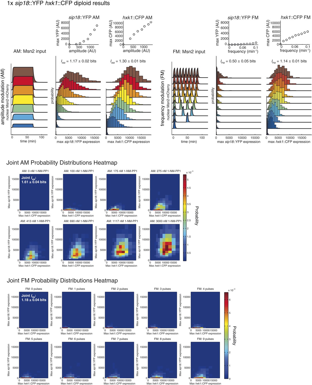
Summary of results for 1× reporter diploid.
This figure shows single and joint distribution histograms for the 1× reporter diploid (sip18::YFP hxk1::CFP). Top panel, left: Cells containing both the sip18::YFP and hxk1::CFP reporters were exposed to either no activation or a 70-min pulse of seven increasing amplitudes from ca. 25% (100 nM 1-NM-PP1) to 100% (3 μM 1-NM-PP1) of maximal Msn2-mCherry nuclear localization and single-cell gene expression was monitored. For each single-cell time-trace, YFP expression is converted to a scalar by taking the maximal YFP value after smoothing. For each Msn2-mCherry input (a fit to the raw data is shown on the left [AM: Msn2 input]), the gene expression distribution is plotted as a histogram of the same color on the right for HXK1 and SIP18. The population-averaged dose–response (top) is obtained by calculating the YFP histogram mean for each Msn2 input condition. Top panel, right: Cells containing both the sip18::YFP and hxk1::CFP reporters were exposed to either no activation or from one to nine 5-min pulses of Msn2-mCherry nuclear localization (ca. 75% of maximal nuclear Msn2-mCherry, 690 nM 1-NM-PP1) at increasing frequency. All calculations were performed as described above. Middle panel: The discretized joint AM distribution is shown with sip18::YFP on the y-axis and hxk1::CFP on the x-axis. The color of each bin corresponds to the probability—dark blue means unoccupied and red corresponds to the highest probability. The single-cell time-traces were converted to scalars as illustrated in Figure 2—figure supplement 1B. Each individual subplot corresponds to a different condition (Msn2 amplitude) and the data have been binned such that the low expression bins are much smaller and therefore harder to see on the plot. Bottom panel: Same as for the joint AM distribution in the middle panel except for the joint FM distribution. Each subplot now corresponds to a specific frequency (and thus number of pulses).
Figure 4—Figure supplement 2
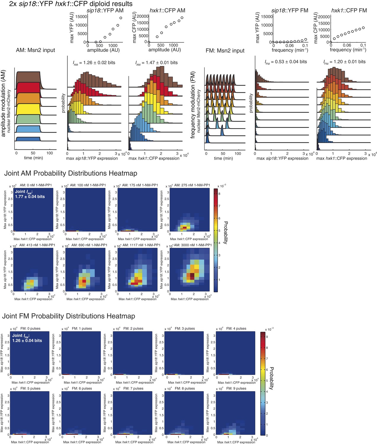
Summary of results for 2× reporter diploid.
This figure shows single and joint distribution histograms for the 2× reporter diploid (2× sip18::YFP 2× hxk1::CFP). Top panel, left: Cells containing both the 2× sip18::YFP and 2× hxk1::CFP reporters were exposed to either no activation or a 70-min pulse of seven increasing amplitudes from ca. 25% (100 nM 1-NM-PP1) to 100% (3 μM 1-NM-PP1) of maximal Msn2-mCherry nuclear localization and single-cell gene expression monitored. For each single-cell time-trace, YFP expression is converted to a scalar by taking the maximal YFP value after smoothing. For each Msn2-mCherry input (a fit to the raw data is shown on the left [AM: Msn2 input]), the gene expression distribution is plotted as a histogram of the same color on the right for HXK1 and SIP18. The population-averaged dose–response (top) is obtained by calculating the YFP histogram mean for each Msn2 input condition. Top panel, right: Cells containing both the 2× sip18::YFP and 2× hxk1::CFP reporters were exposed to either no activation or from one to nine 5-min pulses of Msn2-mCherry nuclear localization (ca. 75% of maximal nuclear Msn2-mCherry, 690 nM 1-NM-PP1) at increasing frequency. All calculations were performed as described above. Middle panel: The discretized joint AM distribution is shown with 2× sip18::YFP on the y-axis and 2× hxk1::CFP on the x-axis. The color of each bin corresponds to the probability—dark blue means unoccupied and red corresponds to the highest probability. The single-cell time-traces were converted to scalars as illustrated in Figure 2—figure supplement 1B. Each individual subplot corresponds to a different condition (Msn2 amplitude) and the data have been binned such that the low expression bins are much smaller and therefore harder to see on the plot. Bottom panel: Same as for the joint AM distribution except for the joint FM distribution. Each subplot now corresponds to a specific frequency (and thus number of pulses).
Author response image 1

Msn2 nuclear localization was simulated with different CVs of Msn2 abundance. Briefly, we assume that Msn2 abundance is gamma distributed and that a given percentage of Msn2 is nuclear for a given inhibitor concentration (e.g. 50% for 275 nM or 75% for 690 nM in accordance with our measurements). The mean Msn2 abundance in the cell was chosen to be 1000 AU. A gamma distribution was then simulated with a and b parameters chosen such that the indicated CV was obtained. Note that the simulation with CV=15% (2.04 bits) closely matches our experimental result (2.06 bits).
Author response image 2
Videos
Video 1
A typical experiment.
Mut B cells were grown in a microfluidic device and exposed to six 5-min Msn2 pulses separated by 10 min and phase contrast (top left), Msn2-mCherry (top right), CFP (bottom left), and YFP (bottom right) reporter expression monitored. Video 1 consists of 64 frames at 2.5 min resolution and images have been compressed, cropped, and contrast adjusted, but not corrected for photobleaching.
Tables
Table 1
List of strains.
| Strain | Type | Strain details |
|---|---|---|
| EY0690 | MATa | W303 (trp1 leu2 ura3 his3 can1 GAL+ psi+) (not generated in this study) |
| EY0691 | MATα | W303 (trp1 leu2 ura3 his3 can1 GAL+ psi+) (not generated in this study) |
| EY2808/ ASH89 | MATa | TPK1M164G TPK2M147G TPK3M165G msn4Δ::TRP1 MSN2-mCherry NHP6a-iRFP::kanMX hxk1::mCitrine_V163A-spHIS5 (not generated in this study) |
| EY2809/ ASH90 | MATα | TPK1M164G TPK2M147G TPK3M165G msn4Δ::LEU2 MSN2-mCherry NHP6a-iRFP::kanMX hxk1::SCFP3A-spHIS5 (not generated in this study) |
| EY2810/ ASH91 | Diploid | TPK1M164G TPK2M147G TPK3M165G msn4Δ::TRP1/LEU2 MSN2-mCherry NHP6a-iRFP::kanMX hxk1::mCitrineV163A/SCFP3A-spHIS5 (not generated in this study) |
| EY2811/ ASH92 | MATa | TPK1M164G TPK2M147G TPK3M165G msn4Δ::TRP1 MSN2-mCherry NHP6a-iRFP::kanMX sip18::mCitrine_V163A-spHIS5 (not generated in this study) |
| EY2812/ ASH93 | MATα | TPK1M164G TPK2M147G TPK3M165G msn4Δ::LEU2 MSN2-mCherry NHP6a-iRFP::kanMX sip18::SCFP3A-spHIS5 (not generated in this study) |
| EY2813/ ASH94 | Diploid | TPK1M164G TPK2M147G TPK3M165G msn4Δ::TRP1/LEU2 MSN2-mCherry NHP6a-iRFP::kanMX sip18::mCitrineV163A/SCFP3A-spHIS5 (not generated in this study) |
| EY2964/ ASH139 | MATa | TPK1M164G TPK2M147G TPK3M165G msn4Δ::TRP1 MSN2-mCherry NHP6a-iRFP::kanMX sip18::mCitrine_V163A-HIS3 pSIP18 Mut A 3 STREs |
| EY2965/ ASH140 | MATa | TPK1M164G TPK2M147G TPK3M165G msn4Δ::TRP1 MSN2-mCherry NHP6a-iRFP::kanMX sip18::mCitrine_V163A-HIS3 pSIP18 Mut B 4 STREs |
| EY2966/ ASH188 | MATα | TPK1M164G TPK2M147G TPK3M165G msn4Δ::LEU2 MSN2-mCherry NHP6a-iRFP::kanMX sip18::SCFP3A-HIS3 pSIP18 Mut B 4 STREs |
| EY2967/ ASH189 | Diploid | TPK1M164G TPK2M147G TPK3M165G msn4Δ::TRP1/LEU2 MSN2-mCherry NHP6a-iRFP::kanMX sip18::mCitrine_V163A/SCFP3A-HIS3 pSIP18 Mut B 4 STREs |
| EY2968/ ASH190 | MATα | TPK1M164G TPK2M147G TPK3M165G msn4Δ::LEU2 MSN2-mCherry NHP6a-iRFP::kanMX sip18::SCFP3A-HIS3 pSIP18 Mut A 3 STREs |
| EY2969/ ASH191 | Diploid | TPK1M164G TPK2M147G TPK3M165G msn4Δ::TRP1/LEU2 MSN2-mCherry NHP6a-iRFP::kanMX sip18::mCitrine_V163A/SCFP3A-HIS3 pSIP18 Mut A 3 STREs |
| EY2970/ ASH192 | MATa | TPK1M164G TPK2M147G TPK3M165G msn4Δ::TRP1 MSN2-mCherry NHP6a-iRFP::kanMX sip18::mCitrine_V163A-HIS3 hxk1::URA3 |
| EY2971/ ASH193 | MATα | TPK1M164G TPK2M147G TPK3M165G msn4Δ::LEU2 MSN2-mCherry NHP6a-iRFP::kanMX hxk1::SCFP3A-HIS3 sip18::URA3 |
| EY2972/ ASH194 | Diploid | TPK1M164G TPK2M147G TPK3M165G msn4Δ::TRP1/LEU2 MSN2-mCherry NHP6a-iRFP::kanMX sip18::mCitrine_V163A-HIS3 hxk1::URA3 / hxk1::SCFP3A-HIS3 sip18::URA3 (1x reporter diploid) |
| EY2973/ ASH195 | MATa | TPK1M164G TPK2M147G TPK3M165G msn4Δ::TRP1 MSN2-mCherry NHP6a-iRFP::kanMX sip18::mCitrine_V163A-HIS3 hxk1::SCFP3A-HIS3 |
| EY2974/ ASH196 | MATα | TPK1M164G TPK2M147G TPK3M165G msn4Δ::LEU2 MSN2-mCherry NHP6a-iRFP::kanMX hxk1::SCFP3A-HIS3 sip18::mCitrine_V163A-HIS3 |
| EY2975/ ASH197 | Diploid | TPK1M164G TPK2M147G TPK3M165G msn4Δ::LEU2 MSN2-mCherry NHP6a-iRFP::kanMX 2x hxk1::SCFP3A_JCat-HIS3 2x sip18::mCitrine_V163A-HIS3 (2x reporter diploid) |
Additional files
-
Supplementary file 1
Raw single-cell time-trace data for HXK1 (15259 cells), SIP18 (21242 cells), pSIP18 mut A (18203 cells), pSIP18 mut B (17655 cells), 1× reporter diploid (21236 cells), and 2× reporter diploid (19222 cells). The data are also available from Dryad Digital Repository (Hansen and O'Shea, 2015).
- https://doi.org/10.7554/eLife.06559.014
-
Supplementary file 2
Computation of Mutual Information. Complete description of information theoretical computations and the algorithm.
- https://doi.org/10.7554/eLife.06559.015
Download links
A two-part list of links to download the article, or parts of the article, in various formats.
Downloads (link to download the article as PDF)
Open citations (links to open the citations from this article in various online reference manager services)
Cite this article (links to download the citations from this article in formats compatible with various reference manager tools)
Limits on information transduction through amplitude and frequency regulation of transcription factor activity
eLife 4:e06559.
https://doi.org/10.7554/eLife.06559


