Visual processing of informative multipoint correlations arises primarily in V2
- Weill Cornell Medical College, United States
Figures
Figure 1
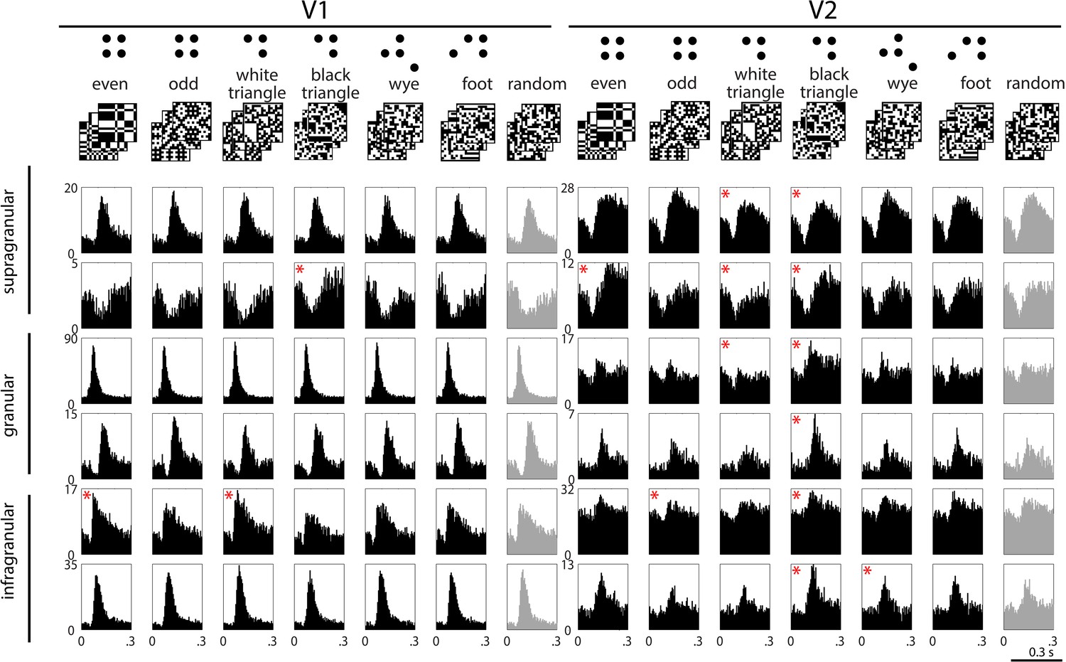
Example responses to multipoint correlations in V1 and V2.
Top row: examples of the stimulus sets used to isolate the different kinds of multipoint correlations. Six sets consist of 1024 16 × 16 binary checkerboards, each with a different statistical structure (left columns); the seventh set consists of 1024 16 × 16 random checkerboards (right column); see ‘Materials and methods’ for details. In each column, the row of PSTH's shows responses of a single neuron to 1024 examples of stimuli drawn from the seven sets. Responses are generally dominated by a transient increase or decrease in firing, occurring 70 to 100 ms after the onset of each stimulus. In some cases, the size or configuration of this transient depends on the type of multipoint correlation (for example, the units in the second row). The asterisks indicate responses to the structured stimulus sets (black) that are significantly different (see ‘Materials and methods’) from the responses to the random stimuli (light gray, beginning of each row). Decremental responses following contrast onset were present in both areas, but more often in V2. However, a decremental response was not a requirement for discriminating among multipoint correlations: outside of supragranular V2, there were many neurons that had incremental responses to the stimulus transient and distinguished among the types of multipoint correlation (for example, the third and fourth rows on the right).
Figure 2 with 1 supplement

Differential sensitivity to multipoint correlations arises intracortically, primarily in V2, and are selective for informative (Tkačik et al., 2010) multipoint correlations.
(A) The multipoint correlation discrimination index (MCDI, see ‘Materials and methods’) for all stimulus types. Upper panels include all neurons in each area, lower three rows subdivide according to lamina. Mean (dark red), median (gray), and 75th percentile (dark green). 25th percentile is 0 in all cases. The red dots in the upper right panel indicate a significant difference between V2 and V1 (p < 0.05, two-tailed, Wilcoxon rank-sum test, false-discovery-rate corrected). The number in the upper left of each panel indicates the number of units analyzed. (B) Mean values of the stimulus-specific MCDI. The stimuli with the highest contributions are the ones that contain correlations that are informative for natural images (Tkačik et al., 2010): even (red), odd (green), white triangles (yellow) black triangles (blue). In contrast, the others (random (black), wye (magenta), and foot (cyan)) are uninformative for natural images, and contributed little to the MCDI. (C) Pairwise discrimination of the multipoint correlation types. The grayscale shows the average pair-specific MCDI, which is the fraction of neurons that respond differentially at any time from 55 to 250 ms following stimulus onset. The stimuli for each row and column are indicated by the same color code as in panel B. Note that panel A shows the overall MCDI, panel B shows the stimulus-specific MCDI, and panel C shows the pair-specific MCDI. (D) Multidimensional scaling of the pair-specific MCDI. The distance between two points corresponds to the fraction of neurons that responds differentially to each type of multipoint correlation. A semitransparent gray plane marks the 0-value along the vertical. Note that in V2, especially in the supragranular layer, there is a wide separation between even and odd stimuli, and between black and white triangle stimuli, and these separations lie on different axes.
Figure 2—figure supplement 1
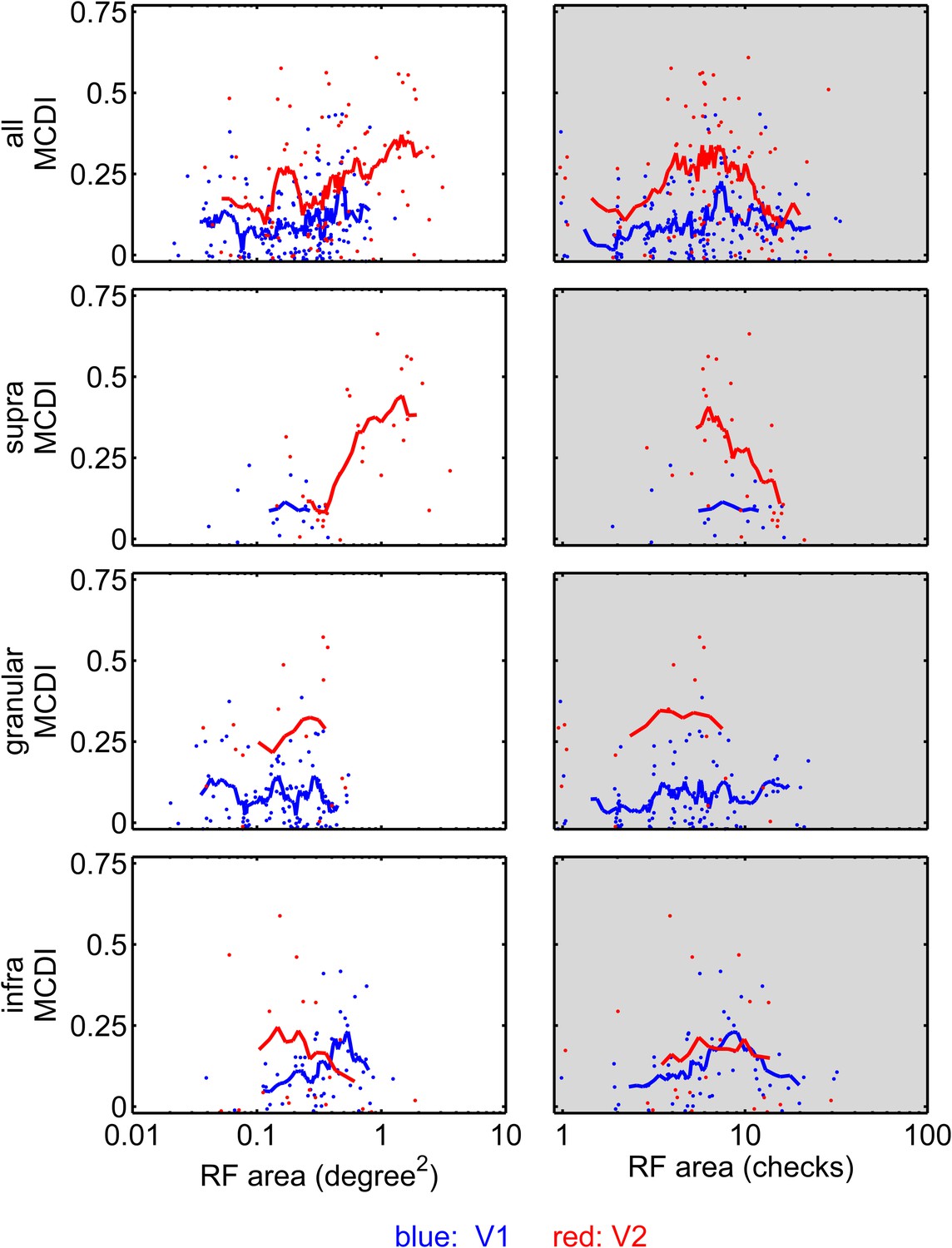
Sensitivity to multipoint correlations in V1 and V2 as a function of RF area and number of checks within the RF.
Each point represents a neuron with a mappable RF (see ‘Materials and methods’): V1 in blue, V2 in red. Left: MCDI as a function of RF area, computed by counting the number of stimulus checks in the RF, and multiplying by the area of each check. Right: MCDI as a function of the number of checks in the RF. The solid lines indicate the moving average of 9 cells, ranked in order shown on the abscissa. Note that when neurons are equated for RF area, either in deg2 or in terms of the number of checks contained, the MCDI is higher in V2 than in V1. This holds across the population and in the supragranular and granular layers. In the infragranular layer, there appears to be a subpopulation of V1 neurons with large RFs and MCDI's that are greater than their counterparts in infragranular V2—though not as great as in granular and supragranular V2.
Figure 3
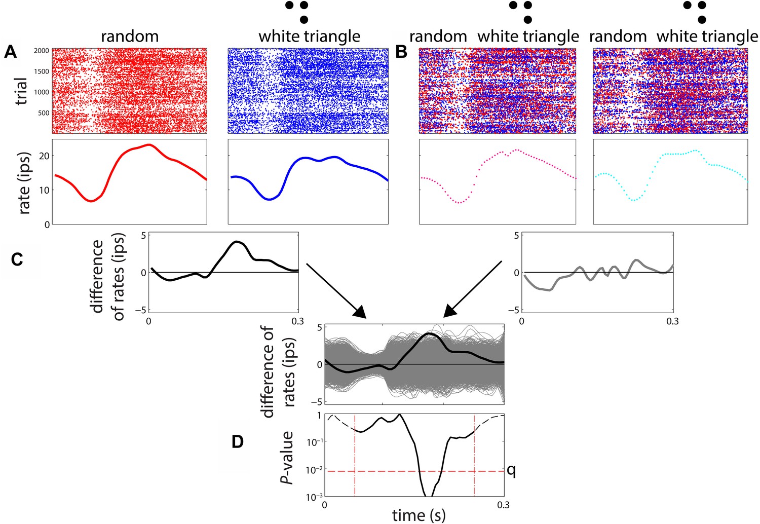
Procedure for determination of differential sensitivity to multipoint correlations for a stimulus pair.
(A) A smoothed firing rate is constructed from the responses to examples of each stimulus type (1024 examples, each presented twice). (B) A parallel procedure is carried out for 3000 surrogate datasets, in which responses are randomly exchanged among the stimuli. The exchanges were limited to responses recorded in adjacent trials, to avoid confounds due to slow change in firing rate over time. (C) The difference between the smoothed responses to the two stimuli is computed, both for the actual responses and each of the surrogate datasets. The relationship of the actual firing rate difference (black) to the distribution of differences encountered in the surrogate datasets (gray) is determined. (D) At each time point, the position of the actual difference in the surrogate difference distribution is expressed as a two-tailed p-value. The actual difference is considered to be significant if any of these p-values over the range 55–250 ms (dashed vertical lines) fall below the false-discovery-rate (FDR) threshold q corresponding to a significance level of 0.05. The FDR threshold q, illustrated as the horizontal dashed line in Figure 3D, is a data-determined quantity (Benjamini and Hochberg, 1995) that is substantially less than the raw significance level of 0.05 (in this case, q < 0.01).
Additional files
-
Source code 1
Custom software written in MATLAB. All computations were done with custom software written in MATLAB (The MathWorks, Inc. MA). In Source code 1, we provide the source code we used for smoothed firing rate computations, computation of the MCDI, statistics, and plotting. Note, though, that much of this code is tied to the specifics of our file formats, naming conventions, etc., and that locfit, used for smoothed firing rate computations, should be downloaded from http://cran.r-project.org/web/packages/locfit/index.html, and compiled for the target system. As mentioned above, spike-sorting was done with Klustakwik and Klusters; these packages can be downloaded from http://klustakwik.sourceforge.net/ (Klustakwik) and http://neurosuite.sourceforge.net/ (Klusters), and then compiled for the target system. Source code 1 is also held on figshare under doi: 10.6084/m9.figshare.1409463.
- https://doi.org/10.7554/eLife.06604.006
Download links
A two-part list of links to download the article, or parts of the article, in various formats.
Downloads (link to download the article as PDF)
Open citations (links to open the citations from this article in various online reference manager services)
Cite this article (links to download the citations from this article in formats compatible with various reference manager tools)
Visual processing of informative multipoint correlations arises primarily in V2
eLife 4:e06604.
https://doi.org/10.7554/eLife.06604


