Mycobacterium ulcerans dynamics in aquatic ecosystems are driven by a complex interplay of abiotic and biotic factors
- Maladies Infectieuses et Vecteurs: Ecologie, Génétique, France
- Ecole des Hautes Etudes en Santé Publique, France
- ecoHEALTH Initiative, Canada
- Réseau International des Instituts Pasteur, Cameroon
- Institut National de la Recherche Médicale U892 (INSERM) et CNRS U6299, équipe 7, France
- International Center for Mathematical and Computational Modelling of Complex Systems (UMI IRD/UPMC UMMISCO), France
Figures
Figure 1 with 1 supplement
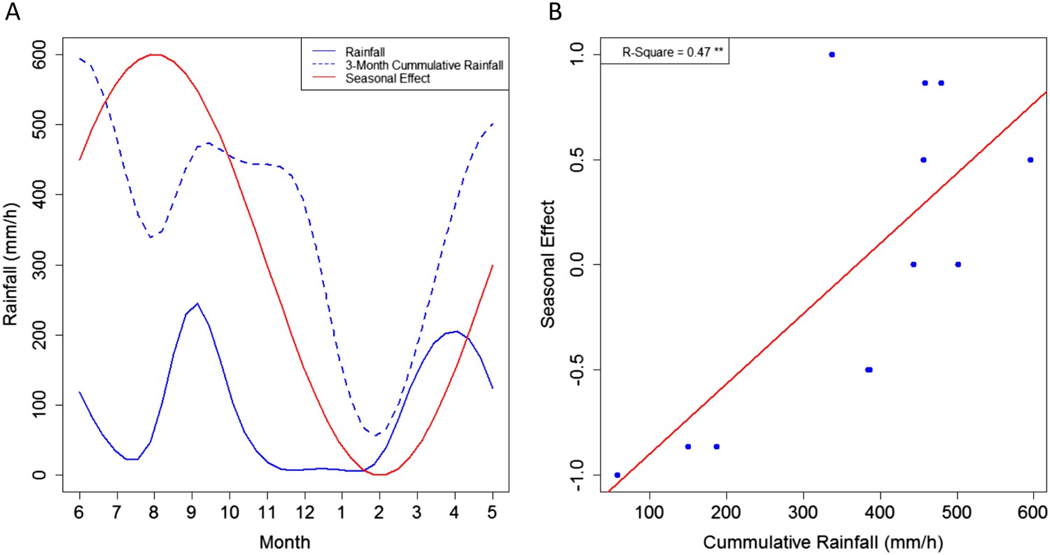
Link between the seasonal effect for M. ulcerans and the rainfall dynamics in Akonolinga.
(A) Represents the monthly values for the seasonal effect (red), the mean rainfall for the period under study and the 3-month cumulative rainfall (blue). (B) Shows a clear linear relationship between the values of the seasonal effect and the 3-month cumulative rainfall. A graphical representation of the different seasonal effects tested can be found in Figure 1—figure supplement 1.
Figure 1—figure supplement 1
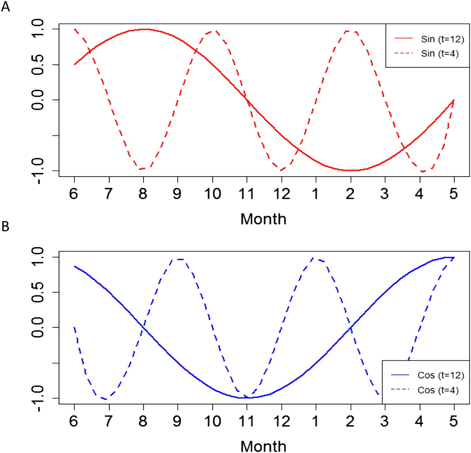
Values for the different seasonal effects tested in the statistical models.
The seasonal effect was tested through sin (A) and cosine (B) functions with frequencies of 12 and 4 months (solid and dashed lines, respectively).
Figure 2
Impact of water flow on physico-chemical characteristics of the water and M. ulcerans prevalence in aquatic communities (Bankim).
(A) Links between water conditions in the first two principal components obtained through principal component analysis (PCA). Comp.1, explaining more than 50% of the variation in physico-chemical conditions in Bankim, reveals that ecosystems with lower water flows have less dissolved oxygen, more acidic pH, and higher temperature. (B) MU positivity in each type of ecosystem as described by the first component of the PCA, which takes into account variations in all physico-chemical characteristics (each category has equal number of points and increasing values of Comp.1). Stagnant ecosystems in Bankim have higher MU positivity than lentic, and these have in turn higher MU positivity than lotic ecosystems. (C) Difference in values for the various water conditions in MU positive and MU negative sites in Bankim. As a result of the association of water flow with the other physico-chemical conditions, similar patterns for MU positivity can be observed for most abiotic conditions.
Figure 3
Distribution of relevant biotic and abiotic variables for Akonolinga and Bankim.
For the construction of histograms (A–D), the relative frequency of the variable within each region is normalized by dividing each frequency by its maximum frequency. It can be noted that the distribution of pH is radically different for both regions, with much more acidic pH in aquatic environments from Akonolinga. For the community composition (E and F), the area an order has in the pie chart is proportional to the mean relative abundance of the order for all sites and months for each region. Only orders representing more than 1% of the overall community are labelled.
Tables
Table 1
Description of environments defined by principal components analysis (PCA) of physico-chemical parameters
| Akonolinga | Bankim | |||||||
|---|---|---|---|---|---|---|---|---|
| PC1 | PC2 | PC3 | PC4 | PC1 | PC2 | PC3 | PC4 | |
| Variance explained | 0.47 | 0.31 | 0.14 | 0.09 | 0.59 | 0.22 | 0.13 | 0.07 |
| Loadings | ||||||||
| pH | −0.33 | 0.7 | −0.47 | 0.41 | −0.51 | 0.51 | −0.43 | 0.55 |
| Dissolved oxygen | −0.6 | 0.31 | 0.31 | −0.67 | −0.57 | 0.33 | 0.11 | −0.75 |
| Water flow | −0.59 | −0.32 | 0.46 | 0.59 | −0.51 | −0.29 | 0.72 | 0.36 |
| Temperature | 0.43 | 0.55 | 0.69 | 0.19 | 0.4 | 0.74 | 0.53 | 0.1 |
-
Separate PCA was performed for Akonolinga and Bankim, and only the most potentially relevant parameters were included.
Table 2
Results from multi-model selection for Akonolinga (12 months of sampling)
| Variable | Avg. effect (b) | Uncond. SE | Lower CL | Upper CL | Relative importance (wi) | Nb. models |
|---|---|---|---|---|---|---|
| (Intercept) | 2.71 | 4.04 | −5.21 | 10.63 | 1.00 | 39 |
| Seasonality | ||||||
| Sine (2pi*Month/12) | 0.36 | 0.16 | 0.04 | 0.67 | 1.00 | 39 |
| Sine (2pi*Month/4) | – | – | – | – | – | – |
| Cosine (2pi*Month/12) | – | – | – | – | – | – |
| Cosine (2pi*Month/4) | – | – | – | – | – | – |
| Physico-chemical parameters | ||||||
| pH | 7.15 | 2.34 | 2.56 | 11.73 | 0.44 | 17 |
| Flow | – | – | – | – | – | – |
| Temperature | – | – | – | – | – | – |
| Dissolved oxygen | – | – | – | – | – | – |
| Conductivity | – | – | – | – | – | – |
| Iron | – | – | – | – | – | – |
| Physico-chemical parameters (PCA) | ||||||
| PC2 | 0.49 | 0.14 | 0.21 | 0.76 | 0.56 | 22 |
| PC1 | – | – | – | – | – | – |
| PC3 | – | – | – | – | – | – |
| Community | ||||||
| Abundance | −0.71 | 0.18 | −1.07 | −0.35 | 1.00 | 39 |
| Shannon | – | – | – | – | – | – |
| Aquatic taxa (%) | ||||||
| Gastropoda | −0.58 | 0.17 | −0.92 | −0.24 | 1.00 | 39 |
| Oligochaeta (Presence) | 0.40 | 0.28 | −0.14 | 0.95 | 0.92 | 36 |
| Odonata | 0.08 | 0.15 | −0.21 | 0.37 | 0.87 | 34 |
| Hydracarina | 0.19 | 0.29 | −0.39 | 0.76 | 0.85 | 33 |
| Trichoptera | −0.01 | 0.16 | −0.31 | 0.30 | 0.67 | 26 |
| Decapoda (Presence) | −1.10 | 0.38 | −1.84 | −0.35 | 0.59 | 23 |
| Hirudinea (Presence) | 0.48 | 0.26 | −0.02 | 0.99 | 0.59 | 23 |
| Coleoptera | 0.24 | 0.20 | −0.15 | 0.63 | 0.54 | 21 |
| Hemiptera | −0.54 | 0.21 | −0.94 | −0.13 | 0.54 | 21 |
| Anura | −0.41 | 0.16 | −0.73 | −0.09 | 0.41 | 16 |
| Ephemeroptera | 0.07 | 0.15 | −0.21 | 0.36 | 0.21 | 8 |
| Diptera | −0.07 | 0.15 | −0.38 | 0.23 | 0.10 | 4 |
-
Variables within each category are ordered by their relative importance. Variables with their 95% confidence interval (CI) with the same sign are represented in bold. Rare aquatic taxa are introduced in the model as Presence/Absence variables, while relative abundance is used for more abundant taxa.
Table 3
Results from multi-model selection for Bankim (4 months of sampling)
| Variable | Avg. effect (b) | Uncond. SE | Lower CL | Upper CL | Relative importance (wi) | Nb. Models |
|---|---|---|---|---|---|---|
| (Intercept) | −13.98 | 4.13 | −22.07 | −5.89 | 1.00 | 100 |
| Seasonality | ||||||
| Sine (2pi*Month/12) | – | – | – | – | – | – |
| Sine (2pi*Month/4) | – | – | – | – | – | – |
| Cosine (2pi*Month/12) | – | – | – | – | – | – |
| Cosine (2pi*Month/4) | – | – | – | – | – | – |
| Physico-chemical parameters | ||||||
| Water flow (lentic) | −1.80 | 0.63 | −3.04 | −0.56 | 1.00 | 100 |
| Water flow (lotic) | −3.63 | 0.88 | −5.35 | −1.91 | 1.00 | 100 |
| pH | – | – | – | – | – | – |
| Temperature | – | – | – | – | – | – |
| Dissolved oxygen | – | – | – | – | – | – |
| Conductivity | – | – | – | – | – | – |
| Iron | – | – | – | – | – | – |
| Physico-chemical parameters (PCA) | ||||||
| PC3 | 0.44 | 0.39 | −0.33 | 1.21 | 0.07 | 7 |
| PC2 | 0.34 | 0.41 | −0.47 | 1.15 | 0.03 | 3 |
| PC1 | 0.67 | 0.33 | 0.03 | 1.32 | 0.01 | 1 |
| Community | ||||||
| Abundance | 0.86 | 0.47 | −0.06 | 1.79 | 1.00 | 100 |
| Shannon | 4.29 | 1.21 | 1.93 | 6.66 | 1.00 | 100 |
| Aquatic taxa (%) | ||||||
| Gastropoda | −0.39 | 0.30 | −0.97 | 0.18 | 0.90 | 90 |
| Anura | −0.54 | 0.37 | −1.26 | 0.19 | 0.89 | 89 |
| Trichoptera | −0.05 | 0.64 | −1.30 | 1.20 | 0.89 | 89 |
| Odonata | −0.05 | 0.30 | −0.63 | 0.53 | 0.87 | 87 |
| Fish | −0.89 | 0.56 | −1.98 | 0.20 | 0.86 | 86 |
| Coleoptera | −0.04 | 0.35 | −0.73 | 0.65 | 0.84 | 84 |
| Diptera | 0.70 | 0.49 | −0.26 | 1.66 | 0.84 | 84 |
| Hirudinea (Presence) | −0.41 | 0.43 | −1.25 | 0.44 | 0.69 | 69 |
| Hydracarina | −1.42 | 0.55 | −2.50 | −0.33 | 0.58 | 58 |
| Decapoda (Presence) | 1.76 | 1.23 | −0.66 | 4.17 | 0.53 | 53 |
| Hemiptera | −0.07 | 0.33 | −0.72 | 0.57 | 0.22 | 22 |
| Oligochaeta (Presence) | −0.02 | 0.48 | −0.96 | 0.92 | 0.14 | 14 |
| Ephemeroptera | −0.84 | 0.25 | −1.33 | −0.35 | 0.13 | 13 |
-
Variables within each category are ordered by their relative importance. Variables with their 95% CI with the same sign are represented in bold. Rare aquatic taxa are introduced in the model as Presence/Absence variables, while relative abundance is used for more abundant taxa. Results for lentic and lotic ecosystems represent the decrease in MU respective to stagnant ecosystems.
Table 4
Description of explanatory variables from our environmental data set and their usage in the statistical model
| Variable | Min | Max | Median | Prop. zeros | Prop. NAs | Usage | |
|---|---|---|---|---|---|---|---|
| Physico-chemical parameters | |||||||
| Temperature | 20.9 | 30.2 | 23 | 0 | 0 | – | Raw |
| pH | 4.5 | 7.1 | 5.5 | 0 | 0 | – | Log |
| Dissolved oxygen | 0.01 | 7.6 | 2 | 0 | 0 | – | Log |
| Conductivity | 10.2 | 110.6 | 22.7 | 0 | 0 | – | Log |
| Water flow | 0 | 0.5 | 0.03 | 0.34 | 0.01 | – | Categorical |
| Turbidity | 2 | 250 | 50 | 0.19 | 0.19 | – | Removed |
| Iron | 0 | 10 | – | 0 | 0 | – | Categorical |
| Phosphates | 0 | 250 | – | 0.07 | 0.07 | – | Removed |
| Sulphates | 0 | 600 | – | 0.22 | 0.22 | – | Removed |
| Aquatic community | |||||||
| Abondance | 46 | 10,591 | 686.5 | 0 | 0 | – | Log |
| Shannon | 0.35 | 2.34 | 1.7 | 0 | 0 | – | Raw |
| Aquatic taxa (%) | |||||||
| Fish | 0 | 0.32 | 0 | 0.32 | 0 | Aquatic | Log |
| Anura | 0 | 0.54 | 0 | 0.33 | 0 | Aquatic | Log |
| Gastropoda | 0 | 0.8 | 0 | 0.37 | 0 | Aquatic | Log |
| Bivalvia | 0 | 0.13 | 0 | 0.91 | 0 | Aquatic | Removed |
| Araneae | 0 | 0.3 | 0.01 | 0.01 | 0 | Terrestrial | Removed |
| Decapoda | 0 | 0.59 | 0 | 0.68 | 0 | Aquatic | Dichotomous |
| Odonata | 0 | 0.54 | 0.11 | 0.02 | 0 | Aquatic | Log |
| Ephemeroptera | 0 | 0.78 | 0.16 | 0.03 | 0 | Aquatic | Log |
| Hemiptera | 0 | 0.41 | 0.08 | 0 | 0 | Aquatic | Log |
| Trichoptera | 0 | 0.19 | 0 | 0.35 | 0 | Aquatic | Log |
| Lepidoptera | 0 | 0.12 | 0 | 0.44 | 0 | Terrestrial | Removed |
| Plecoptera | 0 | 0.01 | 0 | 0.92 | 0 | Aquatic | Removed |
| Oligochaeta | 0 | 0.18 | 0 | 0.69 | 0 | Aquatic | Dichotomous |
| Hirudinea | 0 | 0.45 | 0 | 0.58 | 0 | Aquatic | Dichotomous |
| Coleoptera | 0.01 | 0.94 | 0.1 | 0 | 0 | Aquatic | Log |
| Diptera | 0 | 0.79 | 0.15 | 0 | 0 | Aquatic | Log |
| Hydracarina | 0 | 0.11 | 0 | 0.31 | 0 | Aquatic | Log |
| Collembola | 0 | 0.06 | 0 | 0.4 | 0 | Terrestrial | Removed |
| Cladocera | 0 | 0.24 | 0 | 0.47 | 0.63 | Aquatic | Removed |
Appendix table 1
Results of multivariate analyses for Akonolinga (12 months of sampling) and Bankim (4 months of sampling)
| Variable | Akonolinga (n = 183) | Bankim (n = 61) | ||||
|---|---|---|---|---|---|---|
| Effect | Std. error | p-value | Effect | Std. error | p-value | |
| Model AIC | 400.7 | – | – | 182.7 | – | – |
| Variance of random effect | 0.20 | – | – | 1.77 | – | – |
| (Intercept) | −12.56 | 4.40 | <0.001 | −7.40 | 1.97 | <0.001 |
| Seasonality | ||||||
| Sine(2pi*Month/12) | 0.34 | 0.14 | 0.02 | – | – | – |
| Sine(2pi*Month/4) | – | – | – | – | – | – |
| Cos(2pi*Month/12) | – | – | – | – | – | – |
| Cos(2pi*Month/4) | – | – | – | – | – | – |
| Physico-chemical parameters | ||||||
| Temperature | – | – | – | – | – | – |
| pH | 8.63 | 2.44 | <0.001 | – | – | – |
| Dissolved oxygen | – | – | – | – | – | – |
| Conductivity | – | – | – | – | – | – |
| Iron | – | – | – | – | – | – |
| Water flow (Lentic) | – | – | – | −2.10 | 0.47 | <0.001 |
| Water flow (Lotic) | – | – | – | −3.18 | 0.69 | <0.001 |
| Physico-chemical parameters (PCA) | ||||||
| PC1 | – | – | – | – | – | – |
| PC2 | – | – | – | – | – | – |
| PC3 | – | – | – | – | – | – |
| Community | ||||||
| Abundance | −0.64 | 0.17 | <0.001 | – | – | – |
| Shannon | – | – | – | 4.16 | 0.97 | <0.001 |
| Orders (%) | ||||||
| Fish | – | – | – | −1.62 | 0.35 | <0.001 |
| Anura | −0.34 | 0.14 | 0.02 | −0.84 | 0.32 | 0.01 |
| Gastropoda | −0.64 | 0.16 | <0.001 | – | – | – |
| Decapoda (presence) | −1.37 | 0.37 | <0.001 | – | – | – |
| Odonata | – | – | – | – | – | – |
| Ephemeroptera | – | – | – | −0.94 | 0.21 | <0.001 |
| Hemiptera | −0.47 | 0.20 | 0.02 | – | – | – |
| Tricoptera | – | – | – | – | – | – |
| Oligochaeta (presence) | – | – | – | – | – | – |
| Hirudinea (presence) | 0.59 | 0.23 | 0.01 | – | – | – |
| Coleoptera | – | – | – | – | – | – |
| Diptera | – | – | – | 1.08 | 0.36 | <0.001 |
| Hydracarine | – | – | – | −1.58 | 0.49 | <0.001 |
-
The models used are Binomial regressions with random effect site, selected with forward–backwards procedure (see section 1 for details).
Appendix table 2
Differences in community composition between Akonolinga and Bankim
| Taxonomic group | Relative abundance (%) | Mann–Whitney test | |||
|---|---|---|---|---|---|
| Akonolinga | Bankim | ||||
| Mean | SD | Mean | SD | p-value | |
| Fish | 1.04 | 2.20 | 2.39 | 4.93 | <0.001 |
| Anura | 2.56 | 6.62 | 2.08 | 6.73 | 0.009 |
| Gastropoda | 2.70 | 7.76 | 3.41 | 9.33 | 0.449 |
| Bivalvia | 0.19 | 1.08 | 0.00 | 0.03 | 0.016 |
| Decapoda | 5.36 | 12.37 | 0.90 | 2.78 | 0.010 |
| Odonata | 12.72 | 9.96 | 15.79 | 15.03 | 0.616 |
| Ephemeroptera | 21.77 | 17.22 | 15.56 | 14.74 | 0.010 |
| Hemiptera | 8.15 | 5.85 | 11.84 | 8.55 | <0.001 |
| Tricoptera | 2.62 | 4.20 | 1.23 | 2.23 | 0.011 |
| Hirudinea | 1.29 | 4.76 | 2.63 | 7.31 | 0.005 |
| Oligochaeta | 0.64 | 1.94 | 0.67 | 2.11 | 0.291 |
| Coleoptera | 18.98 | 20.54 | 11.99 | 11.37 | 0.023 |
| Diptera | 17.58 | 14.23 | 23.69 | 16.25 | 0.004 |
| Hydracarine | 0.83 | 1.38 | 0.90 | 1.77 | 0.171 |
-
For each taxon included in the statistical model, the mean and standard deviation (SD) of the relative abundance (%) for each region are given, along with the p-value of a Mann–Whitney test comparing the mean relative abundance in the two regions.
Download links
A two-part list of links to download the article, or parts of the article, in various formats.
Downloads (link to download the article as PDF)
Open citations (links to open the citations from this article in various online reference manager services)
Cite this article (links to download the citations from this article in formats compatible with various reference manager tools)
Mycobacterium ulcerans dynamics in aquatic ecosystems are driven by a complex interplay of abiotic and biotic factors
eLife 4:e07616.
https://doi.org/10.7554/eLife.07616


