A principle of economy predicts the functional architecture of grid cells
- University of Pennsylvania, United States
- Princeton University, United States
Figures
Figure 1
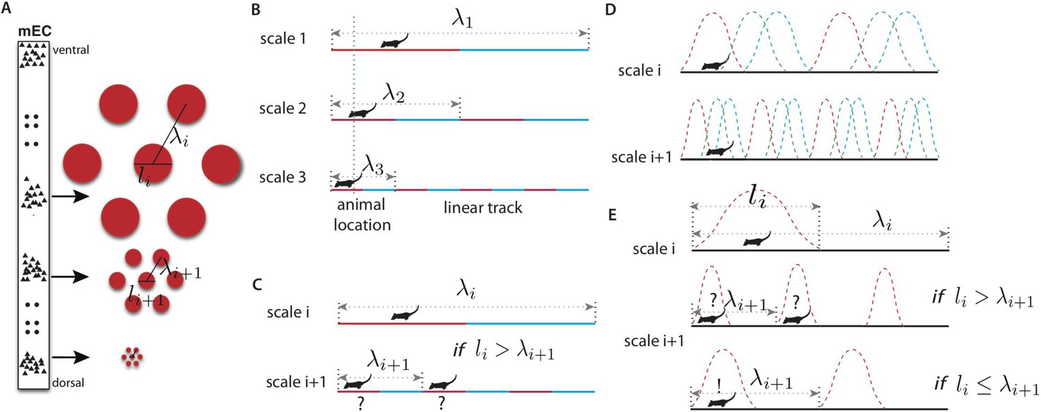
Representing place in the grid system.
(A) Grid cells (small triangles) in the medial entorhinal cortex (MEC) respond when the animal is in a triangular lattice of physical locations (red circles) (Fyhn et al., 2004; Hafting et al., 2005). The scale of periodicity (the ‘grid scale’, λi) and the size of the regions evoking a response above a noise threshold (the ‘grid field width’, li) vary modularly along the dorso-ventral axis of the MEC (Hafting et al., 2005). Grid cells within a module vary in the phase of their spatial response, but share the same period and grid orientation (in two dimensions) (Stensola et al., 2012). (B) A simplified binary grid scheme for encoding location along a linear track. At each scale (λi) there are two grid cells (red vs blue firing fields). The periodicity and grid field widths are halved at each successive scale. (C) The binary scheme in (B) is ambiguous if the grid field width at scale i exceeds the grid periodicity at scale i + 1. For example, if the grid fields marked in red respond at scales i and i + 1, the animal might be in either of the two marked locations. (D) The grid system is composed of discrete modules, each of which contains neurons with periodic tuning curves, and varying phase, in space. (E) For a simple winner-take-all decoder of the grids in panel D, decoded position will be ambiguous unless li ≤ λi + 1, analogously to panel C (see text). Variants of this limitation occur in other decoding schemes.
Figure 2

Trade-off between precision and ambiguity in the probabilistic decoder.
(A) The probability of position x given the responses of all grid cells at scales larger than module i is described by the distribution Qi−1(x) (black curve), and the uncertainty in position is given by the standard deviation δi−1. The probability of position given just the responses in module i will be a periodic function Pi(x) (green curve). (B) The probability distribution over position x after combining module i with all larger scales is Qi(x) ∼ Pi(x)Qi−1(x) and has reduced uncertainty δi. (C) Precision can be improved by increasing the scale factor, thereby narrowing the peaks of Pi(x). However, the periodicity shrinks as well, increasing ambiguity. (D) The distribution over position Qi(x) from combining the modules shown in C. Ambiguity from the secondary peaks leads to an overall uncertainty δi larger than in B, despite the improved precision from the narrower central peak.
Figure 3

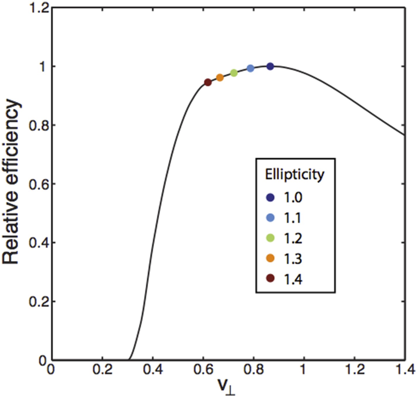
Optimizing two-dimensional grids.
(A) A general two-dimensional lattice is parameterized by two vectors u and v and a periodicity parameter λi. Take u to be a unit vector, so that the spacing between peaks along the u direction is λi, and denote the two components of v by , v⊥. The blue-bordered region is a fundamental domain of the lattice, the largest spatial region that can be unambiguously represented. (B) The two-dimensional analog of the ambiguity in Figure 1C,E for the winner-take-all decoder. If the grid fields in scale i are too close to each other relative to the size of the grid field of scale i − 1 (i.e., li − 1), the animal might be in one of several locations. (C) The optimal ratio r between adjacent scales in a hierarchical grid system in two dimensions for a winner-take-all decoding model (blue curve, WTA) and a probabilistic decoder (red curve). Nr is the number of neurons required to represent space with resolution R given a scaling ratio r, and Nmin is the number of neurons required at the optimum. In both decoding models, the ratio Nr/Nmin is independent of resolution, R. For the winner-take-all model, Nr is derived analytically, while the curve for the probabilistic model is derived numerically (details in Optimizing the grid system: winner-take-all decoder and Optimizing the grid system: probabilistic decoder, ‘Materials and methods’). The winner-take-all model predicts , while the probabilistic decoder predicts r ≈ 1.44. The minima of the two curves lie within each others' shallow basins, predicting that some variability of adjacent scale ratios is tolerable within and between animals. The green and blue bars represent a standard deviation of the scale ratios of the period ratios between modules measured in Barry et al. (2007); Stensola et al. (2012). (D) Contour plot of normalized neuron number N/Nmin in the probabilistic decoder, as a function of the grid geometry parameters after minimizing over the scale factors for fixed resolution R. As in Figure 3C, the normalized neuron number is independent of R. The spacing between contours is 0.01, and the asterisk labels the minimum at ; this corresponds to the triangular lattice.
Figure 4
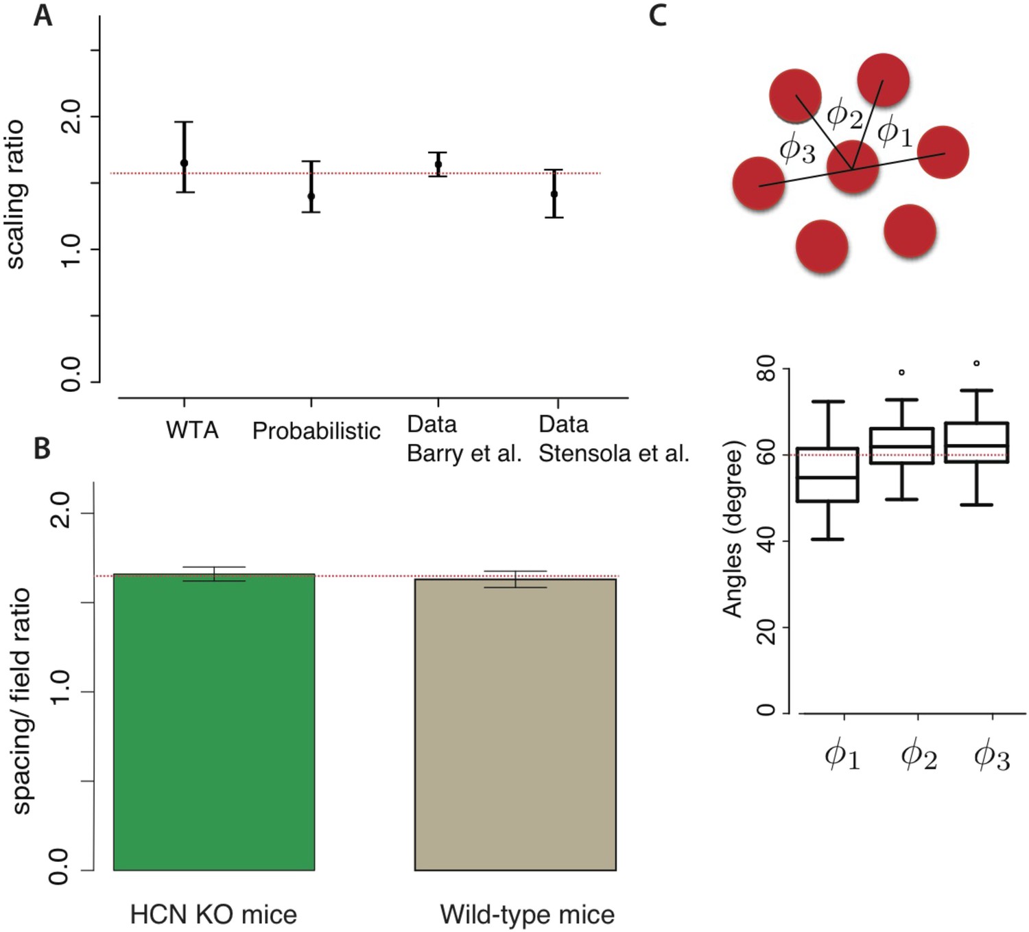
Comparison with experiment.
(A) Our models predict grid scaling ratios that are consistent with experiment. ‘WTA’ (winner-take-all) and ‘probabilistic’ represent predictions from two decoding models; the dot is the scaling ratio minimizing the number of neurons, and the bars represent the interval within which the neuron number will be no more than 5% higher than the minimum. For the experimental data, the dot represents the mean measured scale ratio, and the error bars represent ± one standard deviation. Data were replotted from Barry et al. (2007); Stensola et al. (2012). The dashed red line shows a consensus value running through the two theoretical predictions and the two experimental datasets. (B) The mean ratio between grid periodicity (λi) and the diameter of grid fields (li) in mice (data from Giocomo et al., 2011a). Error bars indicate ± one S.E.M. For both wild-type mice and HCN knockouts (which have larger grid periodicities), the ratio is consistent with (dashed red line). (C) The response lattice of grid cells in rats forms an equilateral triangular lattice with 60° angles between adjacent lattice edges (replotted from Hafting et al., 2005, n = 45 neurons from six rats). Dots represent outliers, as reported in Hafting et al. (2005).
Figure 5
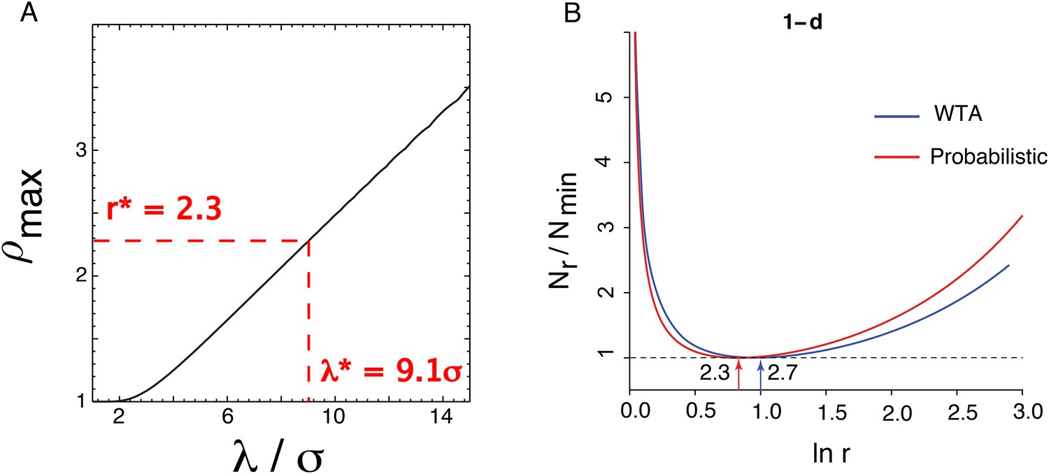
Optimizing the one-dimensional grid system.
(A) is the scale factor after optimizing N over σ/δ. The values r* and λ* are the values chosen by the complete optimization procedure. (B) The optimal ratio r between adjacent scales in a hierarchical grid system in one dimension for a simple winner-take-all decoding model (blue, WTA) and a probabilistic decoder (red). Here, Nr is the number of neurons required to represent space with resolution R given a scaling ratio r, and Nmin is the number of neurons required at the optimum. In both models, the ratio Nr/Nmin is independent of resolution, R. For the winner-take-all model, Nr ∝ r/lnr, while the curve for the probabilistic model is derived numerically (mathematical details in Optimizing the grid system: probabilistic decoder, ‘Materials and methods’). The winner-take-all model predicts r = e ≈ 2.7, while the probabilistic decoder predicts r ≈ 2.3. The minima of the two curves lie within each others' shallow basins.
Appendix figure 1
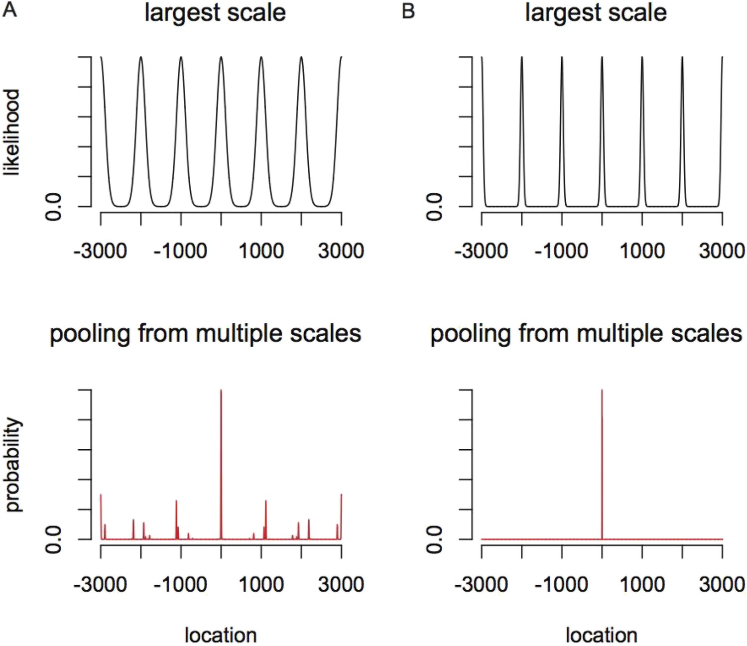
Encoding range can exceed the period of the largest grid module at a cost in the number of neurons.
Assume that the animal is located is at 0. (A) Top, the likelihood resulting from the largest grid module, where the standard deviation of the Gaussian peaks is of the grid period (λmax = 1000). Bottom, the inferred distribution over location after pooling over 4-grid modules related by a scale factor of 2.7. As shown, this 4-module grid system shows ambiguities in location coding outside the range [λmax, λmax]. (B) Top, the likelihood resulting from the largest grid module, where the standard deviation of the Gaussian peaks is of the grid period (λmax = 1000). Bottom, the inferred distribution over location after pooling over four grid modules related by a scale factor of 2.7. As shown, this 4-module grid system provides a good representation over a range of at least [−3000, 3000] = [−3λmax, 3λmax].
Appendix figure 2

The effect of lesioning grid modules on the distribution over location for hierarchical vs non-hierarchical grid schemes.
For the hierarchical scheme, we assume that four one-dimensional grid modules are related by a scale factor r (r = 2.7), that is, , i = 1, 2, 3, and the ratio , i = 1, 2, 3, 4. We assume that the animal is at x = 0 and construct the probability distribution over location given the activity in each grid module as described in Optimizing the grid system: probabilistic decoder, ‘Materials and methods’. For the non-hierarchical scheme, we again assume four grid modules and set the periods of the four modules to be 1/105 (fourth), 1/70 (third), 1/42 (second), 1/30 (first) of the whole range, respectively. We set the width of the composite likelihood after combining all four modules to be 1/210 of the range [−5000, 5000].
Appendix figure 3

The effect of lesioning individual grid modules on place cell activity in a simple grid-place transformation model.
Lesioning different modules leads to qualitatively different effects on the place cell response in the hierarchical coding scheme we proposed, as compared to a non-hierarchical scheme. See ‘Predictions for the effects of lesions and for place cell activity’, Appendix 1 for details.
Author response image 1
Download links
A two-part list of links to download the article, or parts of the article, in various formats.
Downloads (link to download the article as PDF)
Open citations (links to open the citations from this article in various online reference manager services)
Cite this article (links to download the citations from this article in formats compatible with various reference manager tools)
A principle of economy predicts the functional architecture of grid cells
eLife 4:e08362.
https://doi.org/10.7554/eLife.08362


