Normative evidence accumulation in unpredictable environments
Figures
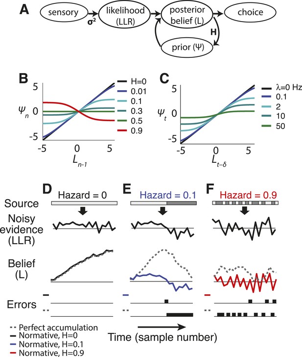
Normative model.
(A) Illustration of the belief-updating process. (B) Discrete-time log-prior odds at a given moment as a function of the belief at the prior moment, plotted as Equation 2 for different values of H. (C) Continuous-time version of the model, with log-prior odds plotted as a function of belief, computed by numerically integrating Equation 4 with dx(t) = 0 over a 16 ms interval. Here expected instability (λ) has units of number of changes per s. Thus, λ → ∞ is analogous to discrete-time H → 0.5. (D–F) Examples of how the normative model (solid lines) and perfect accumulation (dashed gray lines) process a time-dependent stimulus (light vs dark grey for the two alternatives, shown at the top) for different hazard rates (H).
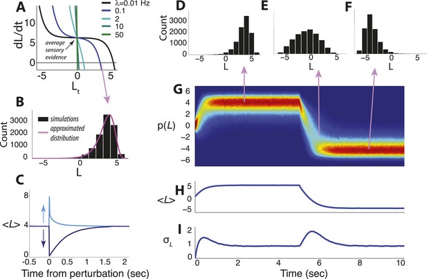
Dynamics of the continuous-time model.
(A) Example of the temporal derivative of belief magnitude plotted as a function of belief magnitude (Equation 4), given an average sensory evidence of 7 units of LLR per unit time. The point of intersection with the dotted line (i.e., derivative = 0) corresponds to the approximate steady-state value of the belief (the mode of the probability distribution). (B) Histogram of belief values at steady state for hazard rate λ = 0.1 Hz from panel A, with the approximated solution in Equation 14a shown in magenta. Note the heavy tail, which is typical for moderate-to-strong input to the model. (C) Asymmetric effects of transient ‘perturbations’ of evidence of equal magnitude (35 units of LLR per s) but opposite signs. Belief magnitude re-converges to steady state faster after the positive perturbation (i.e., favoring the current belief) than the negative perturbation (i.e., opposing the current belief), which accounts for the heavy tail pointed towards zero in B. (D–I) Simulated temporal evolution of the probability distribution of belief value, given an average sensory evidence of 7 units of LLR per s, with an abrupt sign reversal at t = 5 s. (D–F) Histograms of belief at the time-points indicated by arrows. (G) Pseudocolor plot of the full probability distributions normalized by the peak probability over the entire time series. Hot/cold colors indicate high/low probabilities. (H) Expected value of the belief variable. (I) Standard deviation of the belief variable. Note that after a change-point, leaky integration is re-started and beliefs pass through the ‘low-confidence’ regime of the model, resulting in a transient increase of variability that is approximately Gaussian. All simulations used 10,000 iterations.
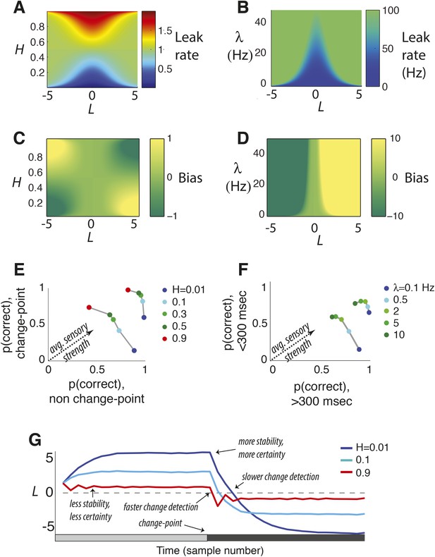
Features of the discrete-time (A, C, E, G) and continuous-time (B, D, F) normative models.
(A, B) Leak rate as a function belief state and hazard rate. Blues are the least leaky and correspond to longer temporal accumulation; reds are the most leaky and correspond to a sign reversal in the change in current belief, resulting in damped oscillations in choice behavior. For the continuous-time model (B), there are no leak rates analogous to discrete-time H > 0.5. (C, D) Bias as a function belief state and hazard rate. Dark greens are the most biased in favor of the alternative associated with negative log-odds; yellows are the most biased in favor of the other alternative. (E, F) Predicted choice accuracy one sample (E) or <300 ms (F) after a change-point vs during steady-state conditions, at different expected hazard rates, as shown, for two difference strengths of evidence (E: |LLR| = 0.5 for leftmost curves and 5 for rightmost; F: |LLR| = 4/s for leftmost curves and 80/s for rightmost). (G) Average belief from the discrete-time model over 1000 simulations for each condition shown, each with a single change-point at trial 20.
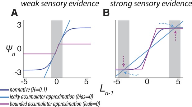
Two ways of approximating the discrete-time normative model, accounting separately for its dynamics when the sensory evidence is consistently weak (A, average |LLR| ≈ 0.25) or strong (B, average |LLR| ≈ 10).
As in Figure 1B, each panel has discrete-time log-prior odds as a function of the belief at the previous moment. Dark blue lines correspond to the normative model for H = 0.1. Light blue lines correspond to a leaky accumulator with no bias, related to the linear approximation in Equation 3a but optimized to best approximate the normative model separately for each average evidence strength in A and B. Magenta lines correspond to perfect accumulation (no leak) to a stabilizing boundary related to Equation 3b,c, also optimized for each evidence strength. In general, the leaky accumulator is better at approximating the normative solution for weak sensory evidence (A), whereas the bounded accumulator is better at approximating the solution for strong sensory evidence (B).
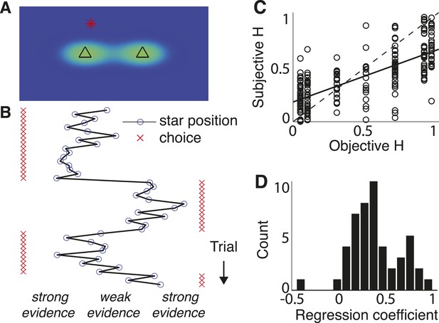
Triangles task and normative model fits.
(A) Example task screen. Triangles and surrounding greenish clouds represent the means and variances of the two generative processes; red star is a single sample (in this case generated by the left process). (B) Sample trials, with actual star position indicated by blue circles and subject choices indicated by red ‘x’. Star positions close to the center represent weak evidence for either of the alternatives because the respective probabilities of either source generating the star position are close. Star positions towards the edge of the screen represent strong evidence for the triangle to which the star is closest. (C) Block-wise subjective (fit) H vs objective H. Dotted line is unity; solid line is a least-squares fit. (D) Histogram of slope coefficients from least-squares fits as in C, calculated for individual subjects.
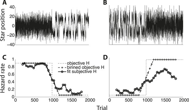
Two examples of subjects adapting to objective hazard rate across an entire experimental session.
(A, B) Star position in arbitrary units plotted as a function of trial number. (C, D) Fit subjective hazard rate (black line with circles) in 400-trial bins slid forward in 50-bin steps, plotted against the median trial number for that bin. Also plotted are the objective hazard rates, unbinned (gray dashed lines) and binned like for the subjective values (black dashed line with hash marks).
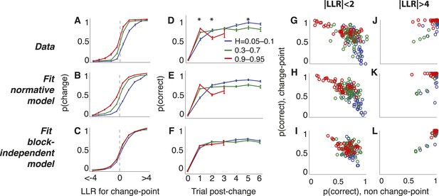
Triangles task choice data pooled across all 48 subjects (top row), plus predictions from fits to the normative model allowing a different subjective hazard rate to be assigned to each block (middle row) and from fits to a model with subjective hazard rates randomly assigned across trials (bottom row).
Colors are different ranges of objective H, as shown in panel D. Errorbars are bootstrapped sem. (A–C) Probability of switching choices as a function of the LLR for a change in the correct answer. Data were restricted to trials following strong evidence (|LLR| > 4) to directly investigate the ‘strong belief’ regime of the model predictions. (D–F) Probability of switching sides in which a strong LLR (|LLR| > 4) for the original side was followed by a change-point and weak (|LLR| < 2) evidence for the opposite side. Significant differences by H in subject data are indicated by asterisks (Bonferroni corrected p < 0.05, χ2 test). (G–L) Block-by-block choice accuracy on change-point vs non-change-point trials when the evidence (magnitude of LLR, as indicated) was relatively weak (G–I) or strong (J–L). Points are individual blocks that included ≥5 trials with the indicated conditions.
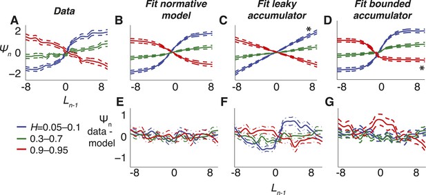
Belief dynamics estimated directly from the data and compared to predictions from the normative model and two suboptimal approximations (Figure 3).
(A–D) Estimates of the log prior-odds on a given trial as a function of belief on the previous trial (compare to Figure 1B) computed for each experimental block, grouped by objective H, as indicated in the legend below panel A. Solid lines are across-block means, and dashed lines are sem. (A) Data. (B) Fit normative model. (C) Fit hazard-dependent leaky accumulator. (D) Fit model with perfect accumulation to a hazard-dependent stabilizing boundary. Asterisks in panels C and D indicate hazard-rate regimes in which estimates from the corresponding model prediction differed significantly from data estimates using Hotelling's t-test with a Bonferroni corrected p < 0.05. (E–G) Hazard-specific differences between the data estimates and model predictions.
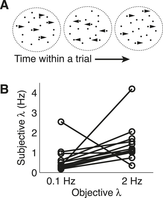
Dots-reversal task and normative model fits.
(A) Representation of a reversing-dots stimulus for a single trial. The subject was instructed to indicate the final, perceived direction of motion. (B) Subjective hazard rate, estimated from direct fits of choice data by the normative model with hazard rate as a free parameter, plotted as a function of objective hazard rate. Each pair of connected points represents data from an individual subject.
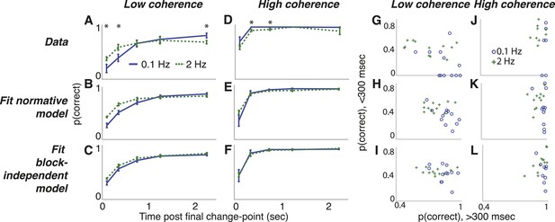
Dots-reversal task choice dynamics comparing the pooled data from 13 subjects (top row) with predictions from fits to the normative model (middle row) and to the normative model with the subjective hazard rates shuffled across trials and blocks for each subject and session (bottom row).
(A–F) accuracy (±bootstrapped sem) as a function of viewing time following the final direction change within a trial for low- (A–C) and high- (D–F) coherence stimuli for the two hazard-rate conditions (indicated in panel A). Asterisks in panels A and D indicate a significant difference between the two hazard-rate conditions (bootstrapped t-test, Bonferroni corrected p < 0.05). (G–L) Dots-reversal task trade-off between accuracy on trials in which the final viewing duration was <300 ms vs >300 ms for different hazard rates (indicated in panel J), when the motion coherence was low (G–I) or high (J–L).
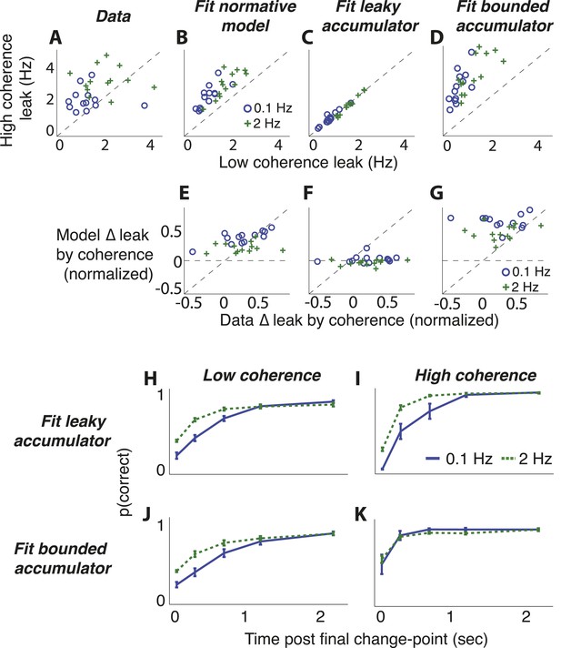
Comparison of predictions from normative model vs from the suboptimal approximations (Figure 3) for the dots-reversal task.
(A–D) Parameter fits from a leaky-accumulator model with separate leak–rate parameters per hazard rate (as indicated in panel B) and coherence (yielding four leaks per subject). (A) Leaks fit to choice data. (B) Leaks fit to predicted choices from the normative model using best-fitting parameters from subject data. (C) Leaks fit to predicted choices from the leaky-accumulator model using leaks that depended on the session-specific hazard rate but not coherence. (D) Leaks fit to predicted choices from the bounded-accumulator model using boundaries that depended on the session-specific hazard rate but not coherence. (E–G) Difference in the best-fitting leak to the two coherences predicted by each of the models above plotted against the difference in leaks from the direct fits to the choice data, separated by hazard rate (see panel B). Differences are normalized by sum of leaks from each of the coherences. In A–G, each point represents a single subject and hazard-rate condition. (H–K) Predicted accuracy (±bootstrapped sem) as a function of viewing time following the final direction change within a trial for low- (H, J) and high- (I, K) coherence stimuli for the two hazard-rate conditions (indicated in panel I), calculated as in Figure 8 but for predictions by fits to the leaky- (H, I) and bounded- (J, K) accumulator models.


