NF-κB oscillations translate into functionally related patterns of gene expression
- San Raffaele Scientific Institute, Italy
- San Raffaele University, Italy
Figures
Figure 1 with 11 supplements

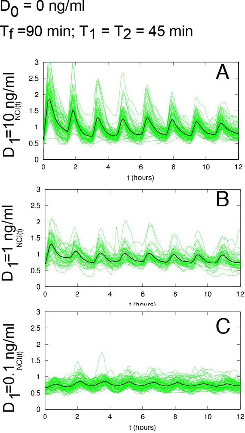
Periodic forcing turns damped heterogeneous oscillation into synchronous sustained oscillations.
(A) The activity of NF-κB is regulated through different negative feedbacks provided by the inhibitors IκB and A20. The scheme at the bottom represents a generic forcing with periodically alternating TNF-α doses D1 and D2 of duration T2+T1 = Tf; Tf is the period of the forcing. (B, C) Oscillations observed in three GFP-p65 cells obtained by computing the nuclear to the cytoplasmic GFP intensity (NCI) for constant flow of 10 ng/ml TNF-α (B) and upon alternating doses D1=10 ng/ml TNF-α, D2=0 ng/ml and T1=T2 =45 min (C). Each colour corresponds to a single cell trace. Oscillatory patterns can be effectively visualised using the phase ϕ of the oscillation, which is 2π in the maxima of the oscillatory peaks (yellow) and π in the local minima (green) in the colour phase-plot of ϕ(t) below the panels. Scale-bar for ϕ is on the right. (D) Time lapse images of cells under constant stimulation displaying the characteristic heterogeneous nuclear-to-cytoplasmic translocations. (E) Phase plot drawn for 50 cells, of 105 analysed, showing the asynchrony of the oscillations except for the first peak. (F) Distribution of the experimentally computed period of the oscillations Texp, measured as the time between two consecutive oscillatory peaks. The distribution has a maximum at T0 =90 min, which corresponds to the natural period. (G) Quantification of the height for each peak. (H) Time lapse images of the cells under periodic stimulation, showing synchronous NF-κB translocations between cytoplasm and nucleus. (I) Phase plot for 50 cells, of 206 analysed, showing a clear synchrony of the oscillations. (J) Distribution of the period of the oscillations Texp. Texp corresponds almost perfectly to the period of the forcing. (K) Quantification of peaks height variation as described in G; values for n>1 are slightly higher than those observed under constant stimulation. Figure supplements from 1 to 10 are provided.
Figure 1—figure supplement 1
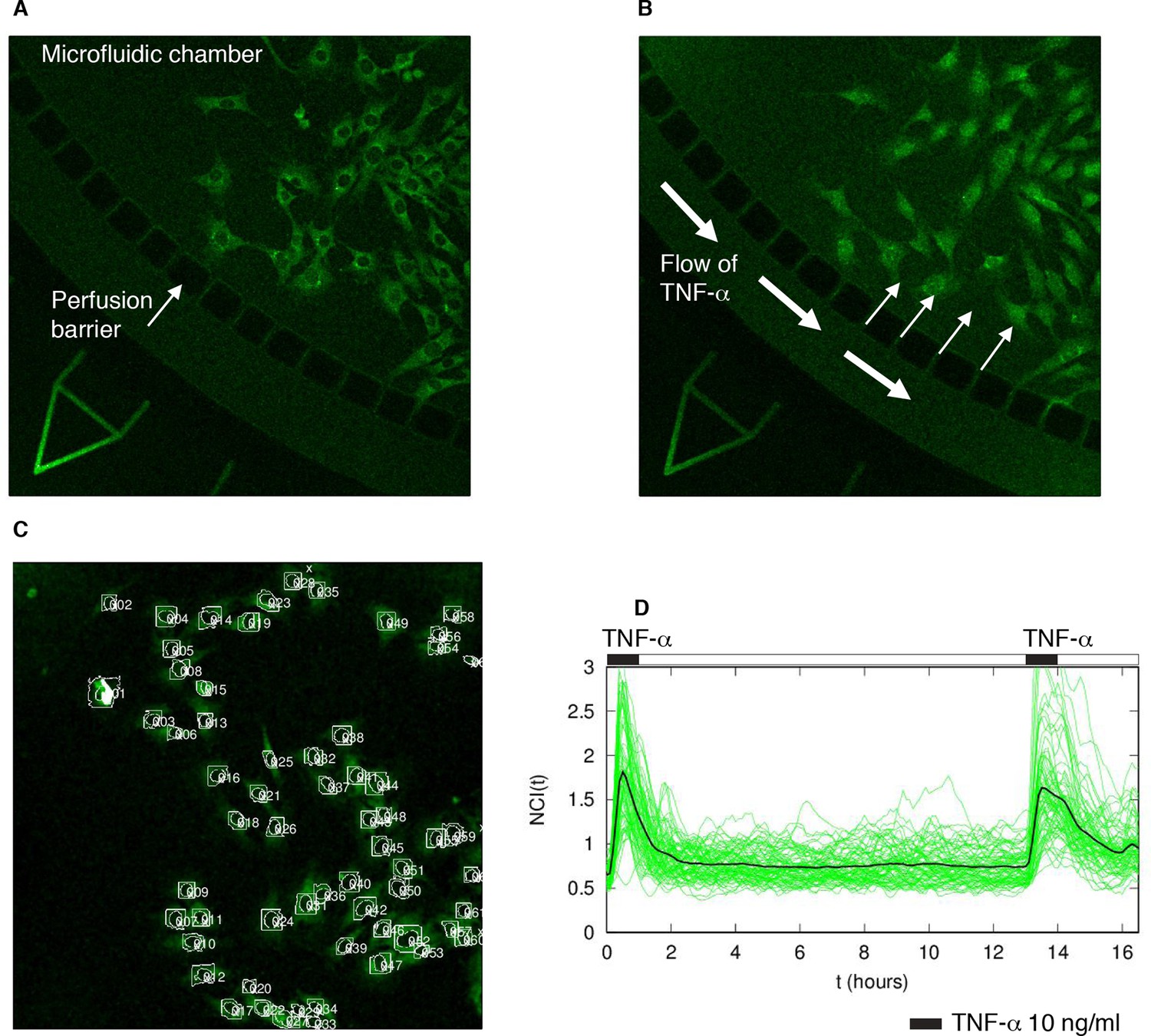
Experimental set-up and quantification.
(A) GFP-p65 MEFs are plated in a microfluidics plate chamber. The perfusion barrier is visible. (B) TNF-α flows and diffuses inside the chamber through the perfusion barrier, minimizing cells’ shear stress. (C) Example of the nuclear segmentation. A square of the cytoplasm around the nucleus is used to compute the nuclear to cytoplasmic ratio of the intensities, an internally normalized measure. (D) The cells were subjected to two pulses of TNF-α of 30 min separated by a washout of 12 hr. The resulting time series shows that cells responded to both pulses with similar intensity, indicating a negligible degradation of TNF-α in our system.
Figure 1—figure supplement 2
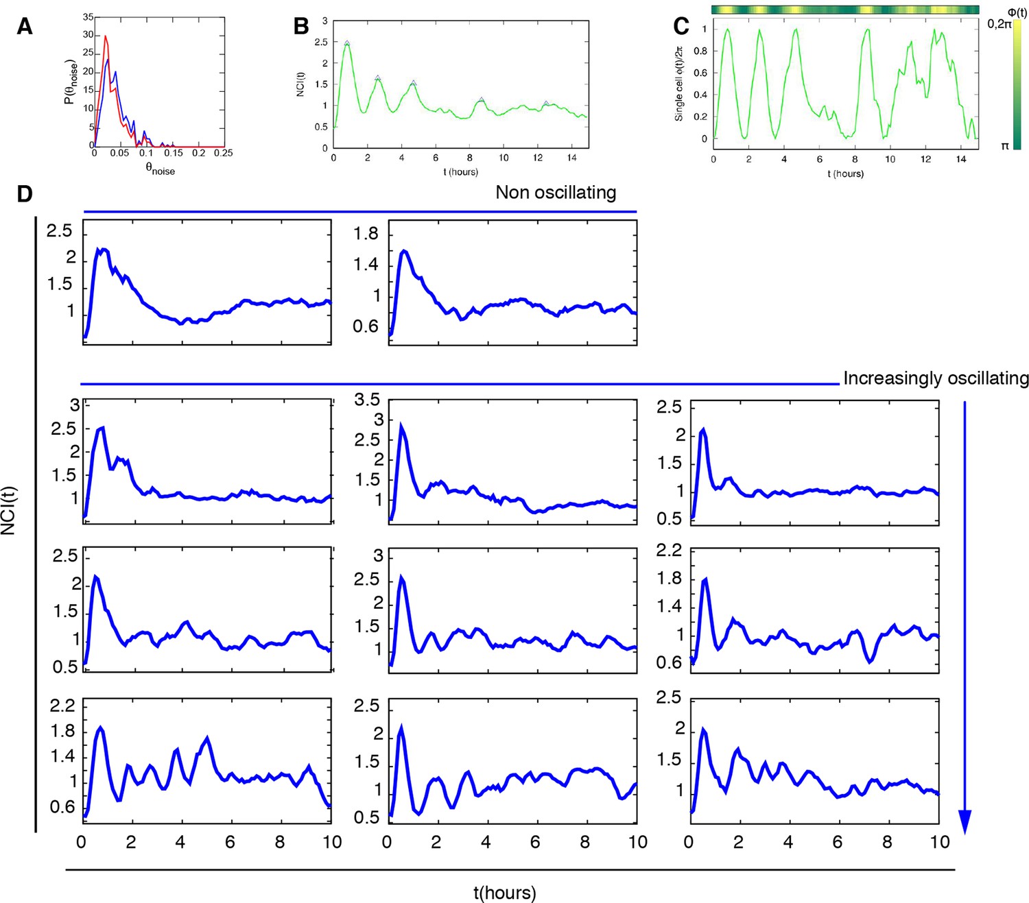
Peaks and phase calculation.
(A) Distribution of the noisy peaks values for unstimulated (blue) and stimulated cells (red). A threshold θ=0.15 is enough to discriminate significant peaks from noisy peaks. (B) Peaks (blue triangles) detected in a typical time series and (C) Phase of the oscillation inferred from the same time series. (D) Selected NCI profiles upon automatic segmentation display a variety of dynamical phenotypes, including the previously oscillating and non oscillating cells.
Figure 1—figure supplement 3
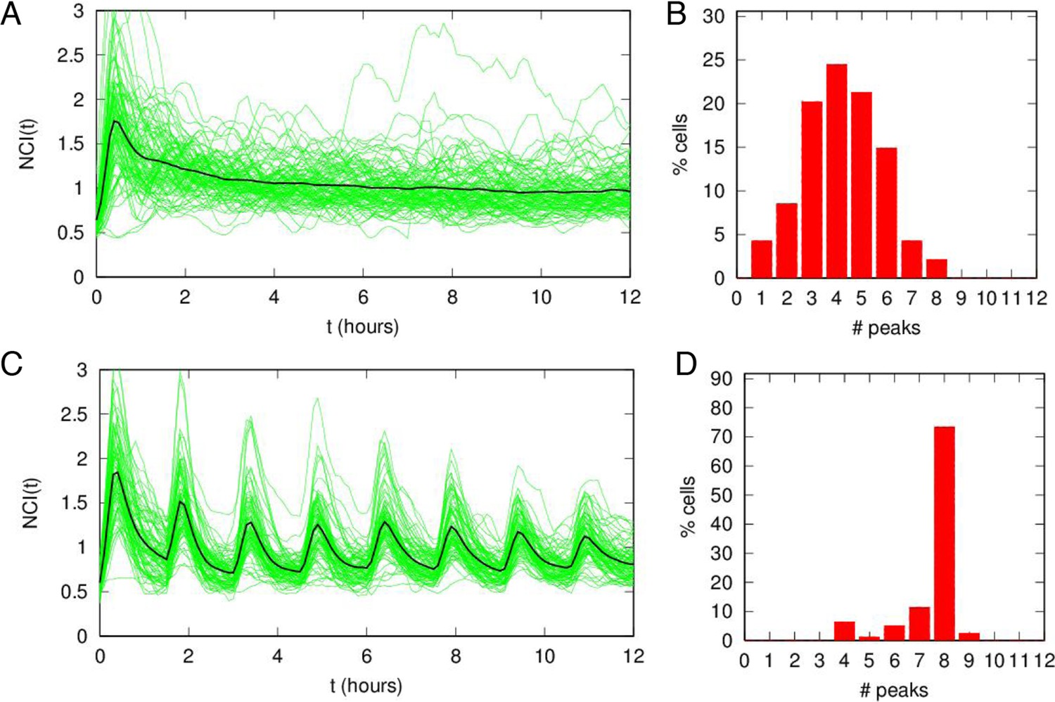
Damped oscillations for constant TNF-α.
(A) NCI (nucleus to cytoplasm intensity) time series (green) and average (black) for cells under a continuous flow of 10 ng/ml TNF-α. Same cells as in Figure 1. (B) Distribution of peak numbers in 12 hr timespan for the cells in A: the average number of peaks (n=4) indicates that there are no sustained oscillations in the 12 hr. (C) NCI time series (green) and average (black) for cells stimulated with repeated pulses of 45 min of 10 ng/ml TNF-α followed by a 45 min wash-out. (D) The average number of peaks of these cells in 12 hr (close to 8) indicates that NF-κB shows sustained oscillations under pulsed stimulation.
Figure 1—figure supplement 4
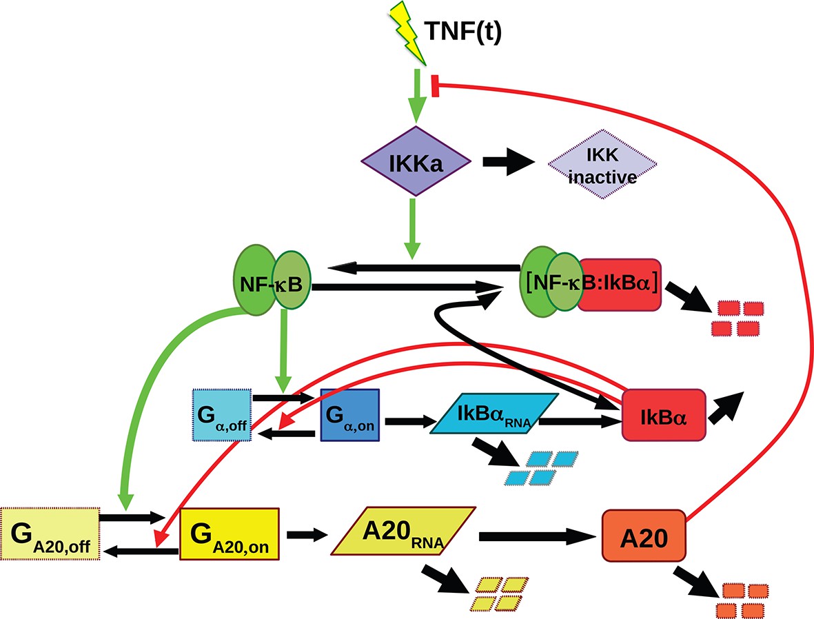
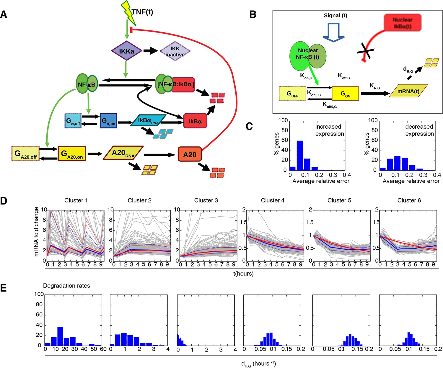
Scheme of the simple ODE mathematical model used for NF-κB dynamics, with the feedbacks provided by IκBα and A20.
Green arrows from NF-κB indicate the contribution of NF-κB to the gene activation while red lines from IκBα represent the contribution to transcriptional repression. The red line from A20 represents the inhibition of IKK activation. This model gives rise to different dynamics for constant stimuli: damped oscillations that converge to a fixed point and sustained oscillations around an unstable fixed point as shown in Figure 1—figure supplement 5.
Figure 1—figure supplement 5
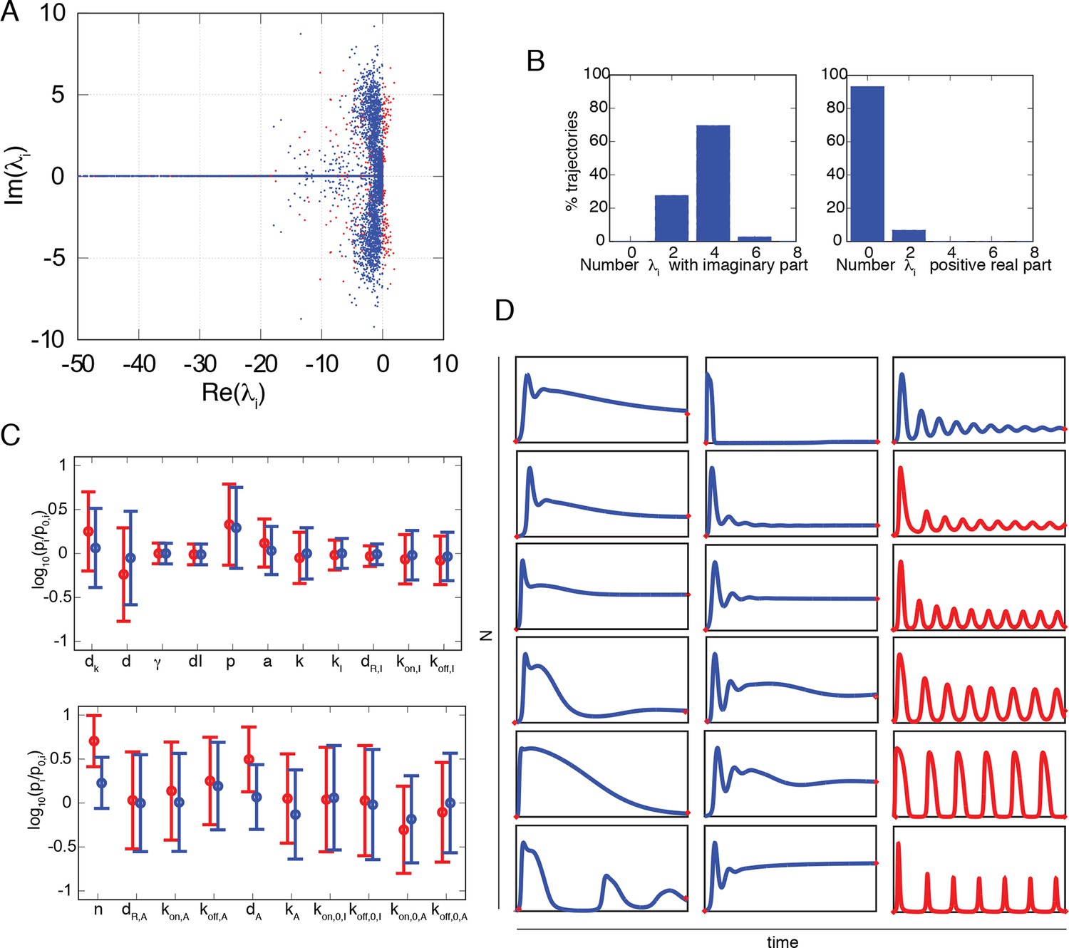
Numerical exploration of the mathematical model suggests that damped oscillations are predominant.
(A) Real and imaginary parts of each eigenvalue of the fixed points of the NF-κB dynamical system. Red dots are for eigenvalues of unstable fixed points, corresponding to sustained oscillations. (B) The distribution of the number of imaginary eigenvalues in fixed points obtained from our set of parameter combinations. Most fixed points have four or more negative eigenvalues, indicating the coexistence of two or more characteristic frequencies. The distribution of the number of positive real parts of eigenvalues in fixed points obtained from our set of parameter combinations. This distribution suggests that sustained oscillations might be infrequent (right). (C) Mean and standard deviation of the parameter values giving rise to oscillating (red) and nonoscillating (blue) trajectories. The intervals are very similar except for parameters n and dA involved in the A20 negative feedback. (D) Examples of the variety of trajectories found in our numerical exploration, including oscillatory trajectories (red) with different peaks and a variety of damped oscillating and non-oscillating dynamics (blue). These computed trajectories are similar to those observed experimentally.
Figure 1—figure supplement 6
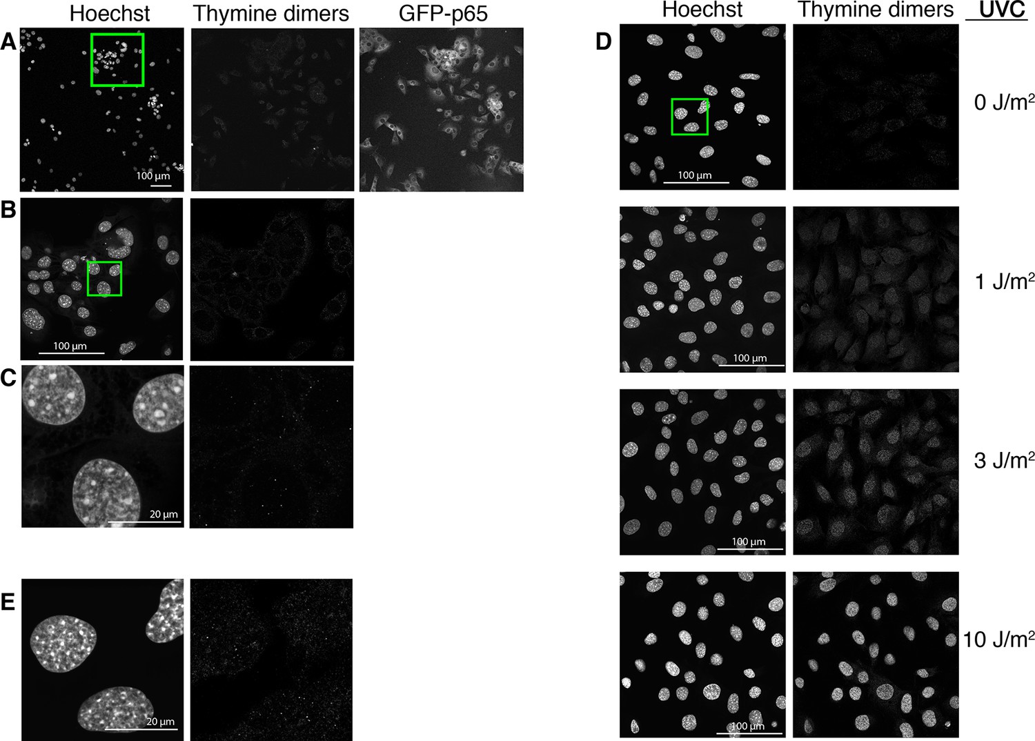
UV-photodamage is not detectable in imaged cells.
The cells were imaged for 15 hr in the presence of Hoechst, fixed and immunostained for thymine dimers (right panel, anti TDM-2 antibody, 20x obj; shown is a representative experiment of three performed). The last image of the GFP-p65 cells acquired at the end of the timelapse acquisition is reported in the middle panel. The green square in the Hoechst panel indicates the area enlarged in panel B. (B) Higher magnification of the selected area in panel A (63x obj). (C) Higher magnification of the selected area in panel B (63x obj, zoom 5). (D) For comparison, GFP-p65 cells were plated in the presence of Hoechst and exposed to increasing doses of UVC and immunostained together with the cells in A. Images were acquired with constant settings in the same microscopy session. Due to the very low intensity, the signal has been enhanced. Fluorescence is almost undetectable in both non-UVC-exposed (0 J/m2) and non-imaged cells (D and B, respectively). (E) Higher magnification of the selected area in panel D (63x obj, zoom 5), green square in 0 J/m2.
Figure 1—figure supplement 7
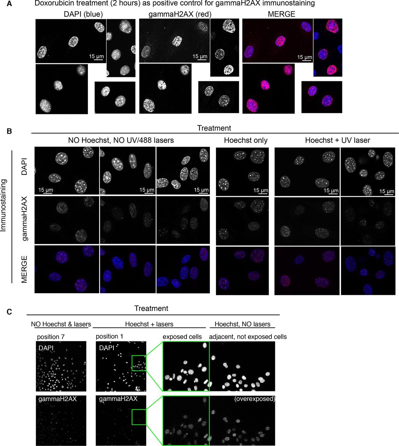
Ongoing DNA repair is not detectable in cells imaged with Hoechst staining and UV irradiation.
Immunostaining for gammaH2AX, a marker indicative of active DNA damage repair, was used to assess genetic damage in unstimulated cells exposed or not to Hoechst staining and UV and/or GFP imaging for 3 hr in microfluidic plates. All the images were acquired during the same microscope session keeping the acquisition parameters rigorously constant. (A) GFP-p65 cells treated with sub-toxic doses of doxorubicin (10 nM) for 2 hrs were used as positive control to set up imaging conditions. Obj: 63x. (B) Left panel contains the negative control: cells cultured in the microfluidic plate were not Hoechst stained, nor UV and GFP imaged. Middle and right panels: immunostaining of cells in microfluidic chambers that were Hoechst-stained but not imaged or both Hoechst-stained and UV-imaged, respectively. Obj: 63x. (C) To further confirm the previous results, and to exclude phototoxicity of the 488 nm laser in GFP imaging, we show fields from a chamber that did not received Hoechst staining and imaging (position 7) or was exposed to both (position 1) in the same experiment (20x Obj). The panel on the right shows an enlargement of a small portion of position 1 (green rectangle) to which the adjacent area outside the imaging field and not exposed to GFP imaging has been added to exclude indirect photodamage (Martin et al., 2005).
Figure 1—figure supplement 8

TNF-dependent activation of apoptosis in GFP-p65 cells stimulated with increasing doses of TNF-α.
Shown is a montage of imaging fields (GFP channel) extracted from representative time-lapse experiments for the indicated time-points. Frame number 0, 10, 30, 60, 90 and 120 correspond to 0, 1, 3, 6, 9 and 12 hr, respectively. Red frames focus on fields with detectable apoptotic cells.
Figure 1—figure supplement 9
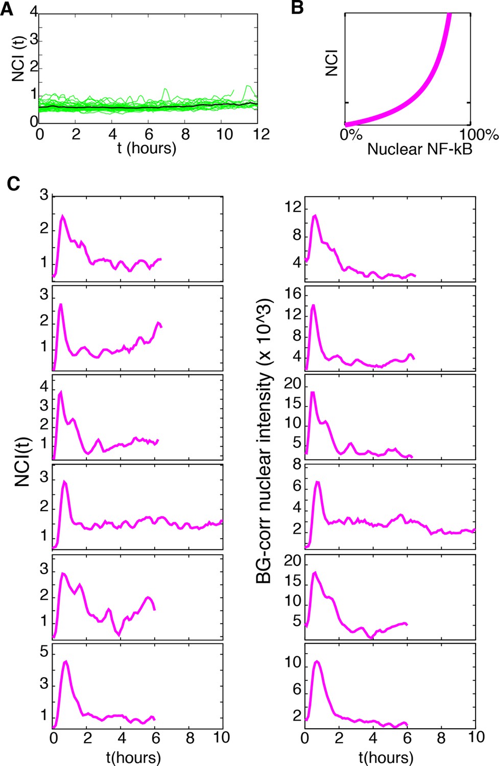
UV and 488 laser imaging does not activate NF-κB nor produce altered NF-κB dynamics.
(A) NCI profiles of untreated cells imaged for 12 hr. (B) Correlation between NCI values and nuclear NF-κB content. (C) Comparison of NCI and background-corrected nuclear intensity profiles obtained by manual segmentation of cells stimulated with 10 ng/ml TNF-α without Hoechst/UV imaging.
Figure 1—figure supplement 10
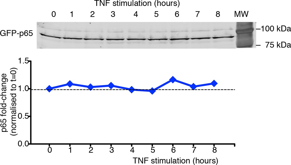
GFP-p65 levels do not change in the cell population upon TNF-α stimulation.
Quantitative immunoblot analysis was performed on cells cultured in 0.1% FCS plus Hoechst and stimulated with TNF-α for the indicated times. Lysates from cells were normalized for their DNA content (De Toma et al., 2014), and the equivalent of 1.5 µg of DNA was loaded per well on 8% SDS-PAGE gels. The 95 kDa band corresponding to the GFP fusion (65 +29 kDa) was detected with anti-p65 antibody (Santa Cruz, Mab, Cat. # sc-372, upper panel) and quantified using the ECL Plex fluorescent western blotting system (GE Healthcare). Sixteen-bit images were acquired with FLA-9000 (Fuji Film); signals were within the linear part of the dynamic range (Celona et al., 2011). Quantification of western blot signals was performed with ImageJ software (Rasband, http://rsb.info.nih.gov/ij). GFP-p65 quantities were expressed as fold change upon setting to 1 the p65 levels in unstimulated cells (bottom panel). Shown is a representative experiment of the three performed. Statistical error: SD of technical replicates (behind symbols).
Figure 1—figure supplement 11
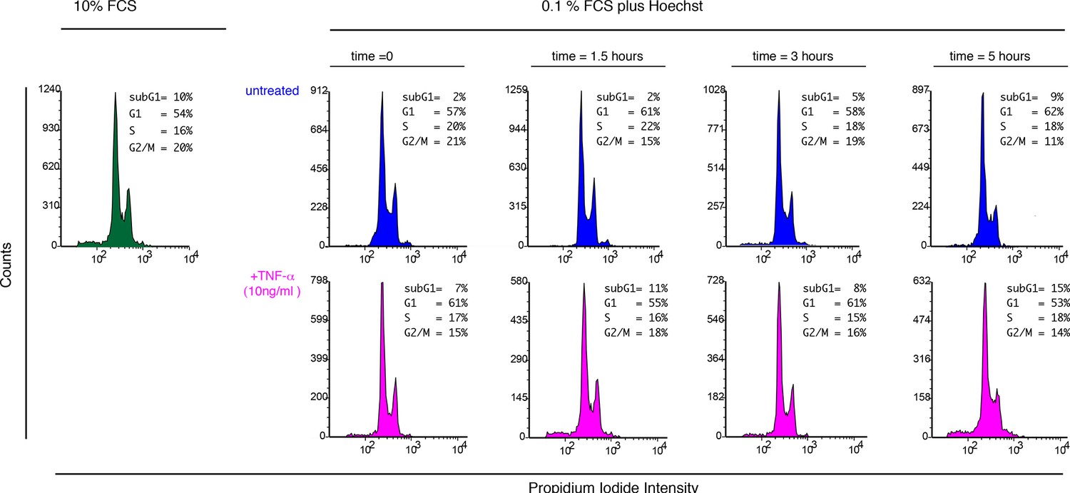
Cell cycle analysis of cells exposed to Hoechst and TNF-α.
To determine whether Hoechst staining might alter the cell cycle, the imaging culture medium (50 ng/ml Hoechst, 0.1% FCS) was added to GFP-p65 MEFs for 2 hr (preincubation). After that time 10 ng/ml TNF-α was added and cells harvested at the indicated timepoints (magenta). For comparison a set of cell samples was left untreated and harvested at the same timepoints (blue ). In green, cells cultured in 10% FCS . Propidium Iodide staining was performed with standard protocols after cell fixation and cells analysed with an Accuri FACS instrument (Becton-Dickinson). The fractions of cells in each cell cycle phase are reported. Shown is one of three representative experiments.
Figure 2 with 3 supplements

Synchronous oscillations arise for different forcing amplitudes.
(A) Representative phase plots for 25 cells (out of 216, 80, 188, 263, 225 cells analysed) stimulated with D1=10, 1, 0.5, 0.25, 0.1 ng/ml TNF-α, D2=0 ng/ml, for Tf =90 min, T1=T2=45 min. (B) Distributions of the periods for the cells shown in panel (A); distributions become narrower as the dose D1 increases. The appearance of a second peak at Texp=3 hr at lower doses means that in some cycles a fraction of cells miss a peak and the interval to the next one is double. (C) Quantification of height of the nth peak in the different conditions considered in (A). By decreasing the stimulus amplitude, the ratio tends to stabilize to a constant value. (D) Distribution of the phase difference Δϕ for the forcings considered: Δϕ becomes narrower as the forcing amplitude is increased. (E) The synchrony intensity η, an entropy-based measure on how widely distributed the values of Δϕ are, increases with the amplitude of D1 for Tf =90 min. (F) The synchrony intensity ηn computed using only the peaks observed in each forcing cycle shows that the synchrony does not increase with the successive cycles of forcing. Figure supplements from 1 to 3 are provided.
Figure 2—figure supplement 1
NCI and average dynamics for different forcings.
NCI of single cell time series (green) and average (black) for the indicated doses, (A) to (C) plots correspond to a forcing of 90 min. Cell numbers as in Figure 2.
Figure 2—figure supplement 2
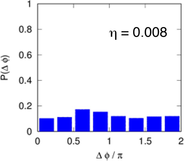
Distribution of the phase differences for cells stimulated with constant TNF-α.
The distribution is almost flat and the synchronization intensity η is very low. Cell numbers as in Figure 1.
Figure 2—figure supplement 3
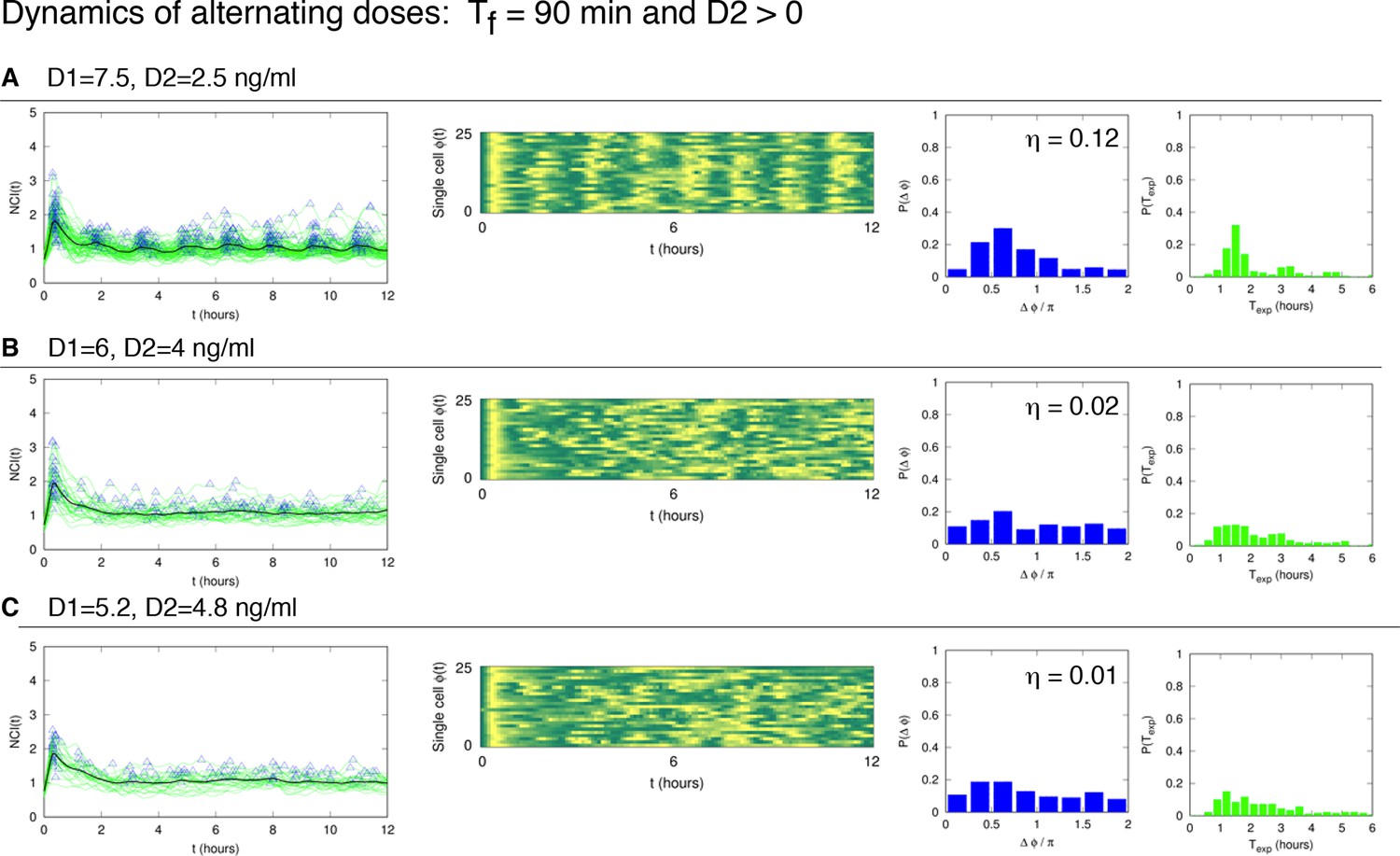
Dynamics of alternating doses Tf = 90 min and D2 > 0.
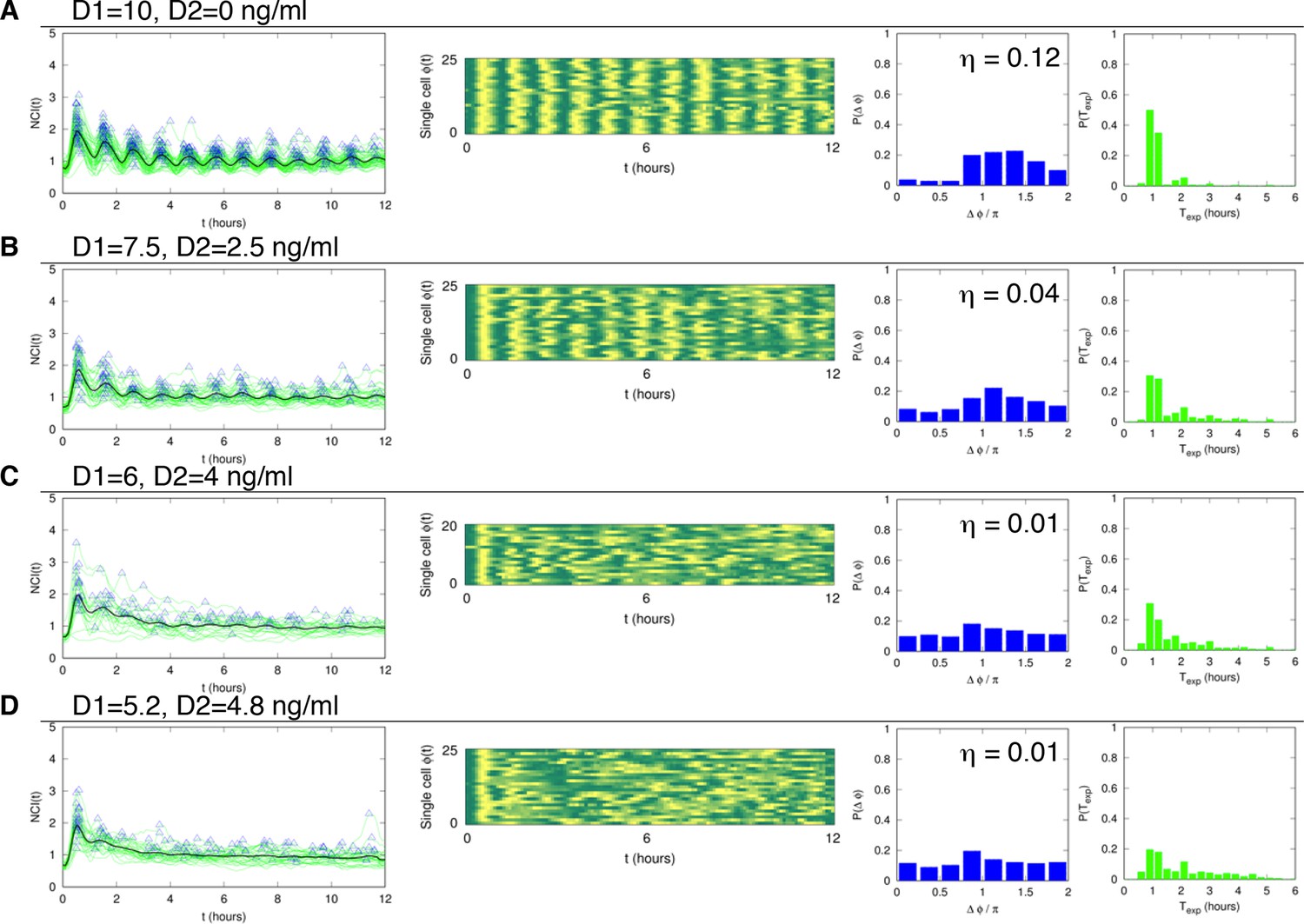
Panels in each row (left to right) represent the single cell NCI dynamics (green) plus the average (black) and the detected peaks (triangles); the phase plot; the phase difference distribution (with the synchrony intensity value η) and the experimental period distribution. (A) D1=7.5, D2=2.5, (B) D1=6, D2=4 and (C) D1=5.2, D2=4.8 (in ng/ml TNF-α). Twentyfive cells are reported in the phase plots out of 111, 78, 66 analysed, respectively. T1 = T2 = 45 min.
Figure 3 with 3 supplements

Cells adjust oscillations to different periods for a wide range of forcing amplitudes.
Representative phase plots for 25 cells stimulated with D1=10, 1, 0.1 ng/ml TNF-α (out of 151, 77, 123 cells analysed, respectively) D2=0 ng/ml for (A) Tf =180 min with T1= 30 min and (B) Tf =45 min with T1=22.5 min (analysed 101, 112, 119 cells). (C, D) Plots showing the distributions of the periods for the conditions given in panels (A) and (B), respectively. (E, F) Average peaks height in the intervals [(n–1) T0, T0) and [(n–1) T0/2, nT0/2), for A and B, respectively. In (E), even n correspond to peaks right after stimulation, odd n correspond to the small peak arising between two consecutive stimulations. (G, H) Distribution of the phase difference Δϕ for the forcings in A and B: Δϕ has narrower distributions for higher doses. (I) The synchrony intensity η grows with the doses for Tf=180 min (blue) and Tf=45 min (red). (J, K) Synchrony intensity plots show that ηn does not increase as successive cycles of forcing are applied to the system, both for Tf=180 min and Tf=45 min, respectively. All the analyses included all the tracked cells with no preselection of the responding ones. Figure supplements 1 to 3 are provided.
Figure 3—figure supplement 1
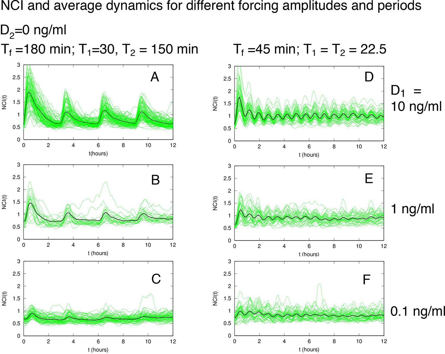
NCI and average dynamics for different forcings.
NCI of single cell time series (green) and average (black) for the indicated doses and timings. (A–C) correspond to a forcing of 180 min, while (D–F) to a forcing of 45 min. D1 is indicated on the right.
Figure 3—figure supplement 2
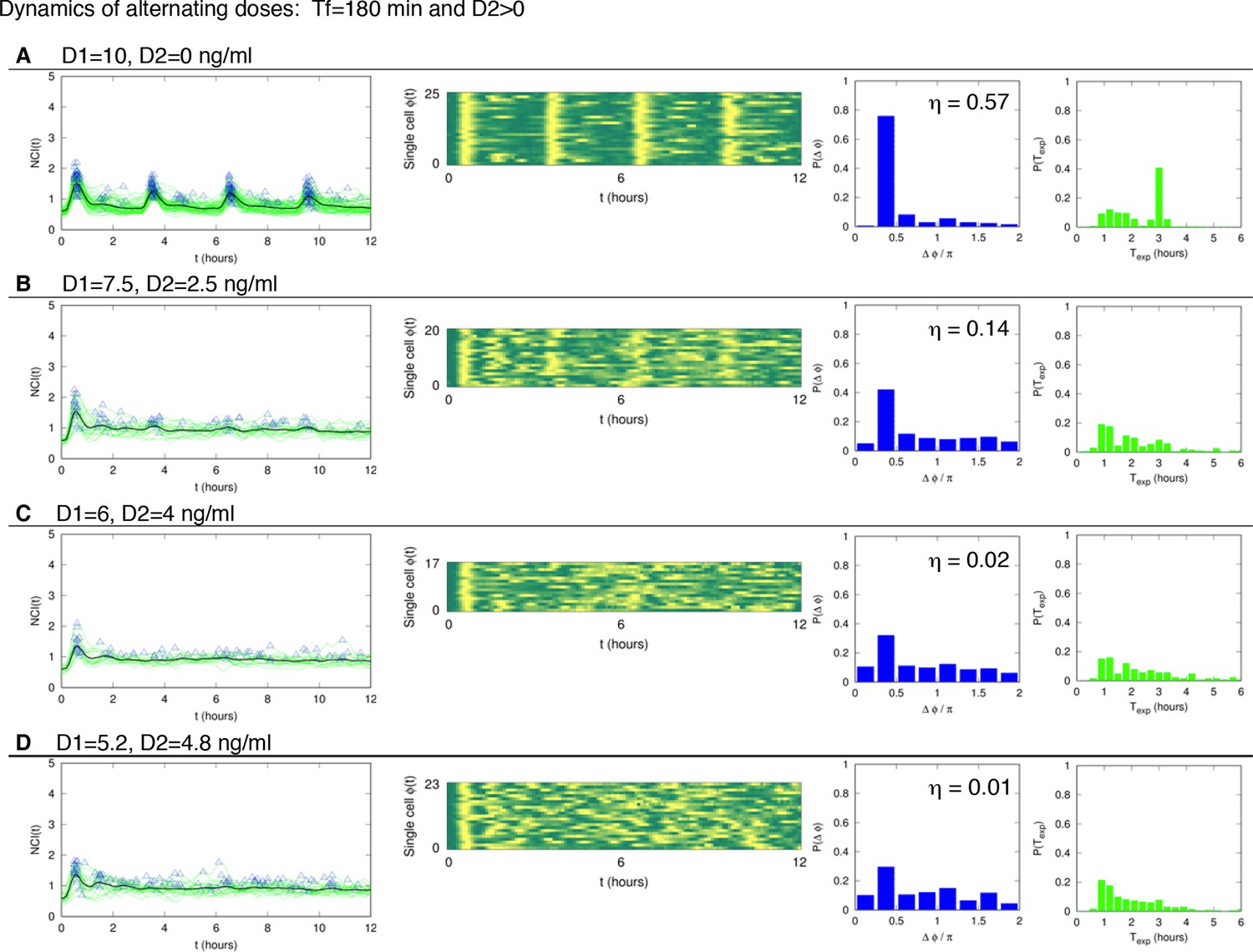
Dynamics of alternating doses Tf=180 min and D2>0.
Panels in each row (left to right) represent the single cell NCI dynamics (green) plus the average (black) and the detected peaks (triangles); the phase plot; the phase difference distribution (with the synchrony intensity value η) and the experimental period distribution. (A) D1=10, D2=0; (B) D1=7.5, D2=2.5; (C) D1=6, D2=4 and (D) D1=5.2, D2=4.8 ng/ml TNF-α. Number of cells analysed: 102, 68, 47, 70, respectively. T1=30 min, T2=150 min.
Figure 3—figure supplement 3
Dynamics for cells synchronised with T1=30 min and different TNF concentrations.
NCI and average dynamics for 45 and 90 min forcing amplitudes, with TNF-α stimulation of 10 and 1 ng/ml, are reported here to integrate results presented in main Figures 2A and 3B. The aim was to assess synchronization for a constant T1 value of 30 min as opposed to 45 and 22 min. Each row shows (A) the phase plots (approximately 150 cells analysed per condition), (B) the single-cell NCI dynamics (green) plus the average (black) and the detected peaks (blue triangles) for a specific condition of synchronization. (C) The experimental period distribution ; (D) the phase difference distribution (with the synchrony intensity value η.
Figure 4 with 4 supplements
Cells do not keep a memory of the synchronous oscillatory dynamics.
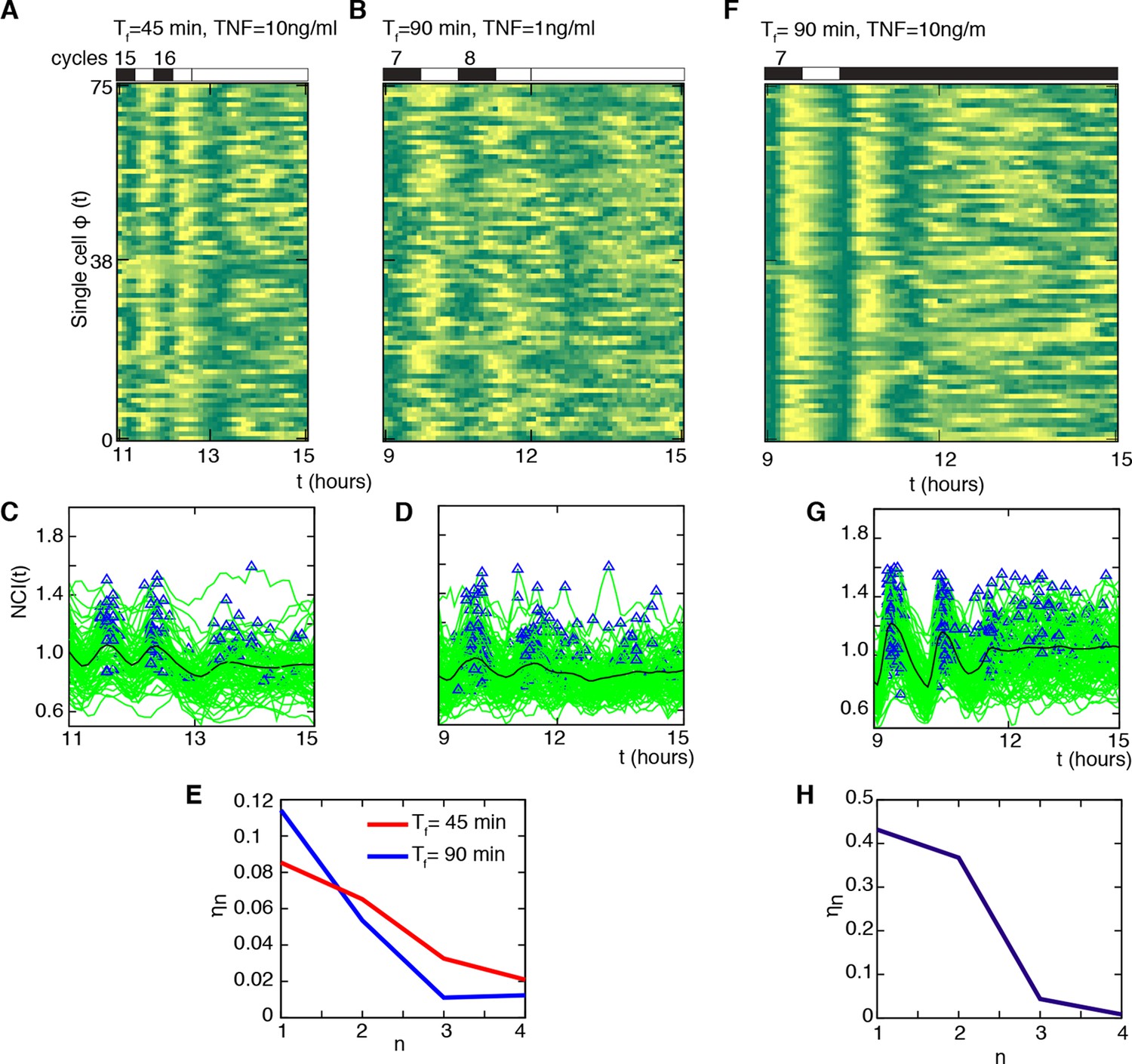
(A, B) Phase plots of the last two oscillation cycles for Tf =45 min (D1=10 ng/ml) and Tf =90 min forcing (D1= 1 ng/ml) (number of forcing cycles are indicated above) followed by a period of 3 hr with no stimulation (75 cells are displayed out of 106 and 197 cells analysed, respectively). (C, D) NCI time series at single cell level (green lines) for the two conditions (A) and (B). Blue triangles indicate the peaks considered in the computing. The thick black line is the average NCI, showing a small peak 90 min after the last forced peak for Tf =45 min (C), compatible with the natural timescale of the free oscillations. (E) The synchrony intensity ηn for the last two forced peaks (n=1, 2) and for the peaks detected in the absence of the stimulus (n=3, 4) illustrates the fast loss of synchrony. (F) Phase plots of the last two oscillation cycles for Tf =90 min (number of forcing cycles are indicated above) (D1=10 ng/ml) followed by 4.5 hr flow of 10 ng/ml TNF-α (75 cells are displayed out of 149 cells analysed). (G) NCI time series at single-cell level (green lines). Blue triangles indicate the peaks considered in the computing. The thick black line is the average NCI, showing a small peak 90 min after the last forced peak, compatible with the natural timescale of the free oscillations. (H) The synchrony intensity ηn for the last two forced peaks (n=1, 2) and for the peaks detected in the presence of the stimulus (n=3,4) illustrates the fast loss of synchrony. Figure supplements from 1 to 4 are provided.
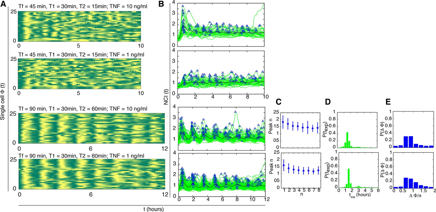
Figure 4—figure supplement 1
Dynamics of alternating doses Tf=60 min and D2>0.
Panels in each row (left to right) represent the single cell NCI dynamics (green) plus the average (black) and the detected peaks (triangle); the phase plot; the phase difference distribution (with the synchrony intensity value η) and the experimental period distribution. (A) D1=10, D2=0; (B) D1=7.5, D2=2.5; (C) D1=6, D2=4 and (D) D1=5.2, D2=4.8 (in ng/ml TNF-α). Analysed cells: 102, 91, 70 and 104, respectively. T1=30 min, T2=30 min.
Figure 4—figure supplement 2
The model predicts that NF-κB oscillations follow the forcing period.
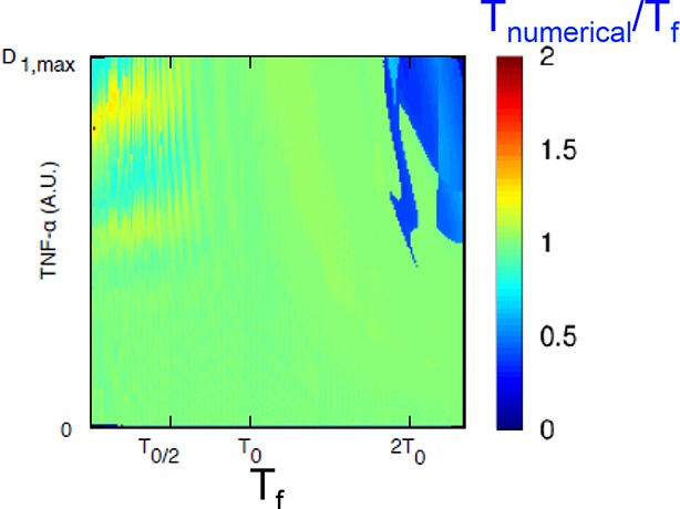
We computed the period to which the NF-κB system converges (average timing between peaks in a 15-hr timespan) for different periods of the forcing and various forcing amplitudes. A representative plot of the results obtained is shown: we keep PNF-κB constant while varying the forcing parameters PS. D1 varies between 0 and Dmax=2 and T1=T2=Tf/2. The ratio Tnumerical/Tf between the computed NF-κB period and the forcing period is very close to one, as expected for damped oscillations when periodically forced. Only for high values of the period the ratio is close to 0.5.
Figure 4—figure supplement 3
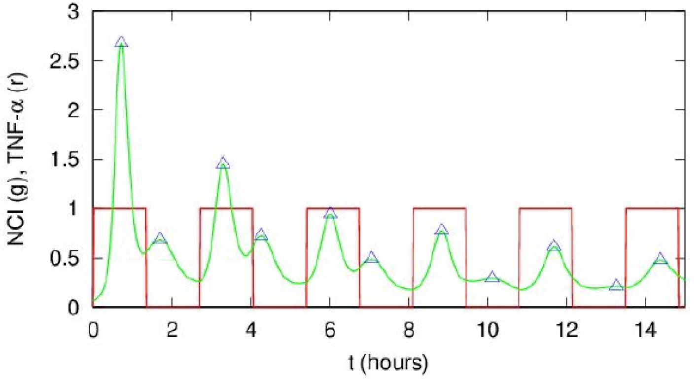
Interpretation of the Tnumerical/Tf ratios close to 0.5 in Figure 4—figure supplement 2.
This ratio is due to the presence of smaller peaks between the bigger post-stimulation peaks in our simulations. An example of our simulations for NCI (green line) and the forcing (red line) is shown. Notice that the smaller peaks tend to decrease in time. This dynamics is reminiscent of the one observed for Tf=2T0=180 min in our experiments, see Figure 3A.
Figure 4—figure supplement 4

Sawtooth-like profiles lead to heterogeneous but synchronous dynamics in GFP-p65 cells.
Each row shows (i) the phase plot for 25 cells ( Approximately 100 cells were analysed per condition), (ii) the single cell NCI dynamics (green) plus the average (black) and the detected peaks (blue triangles), (iii) the experimental period distribution and (iv) the phase difference distribution (with the synchrony intensity value η) for a specific condition ofstimulation with a sawtooth profile, generated by a 15 min pulse followed by no washout. The TNF-α concentrations used are indicated for each row. For forcings of 60 and 90 min we observe synchronization similar to the one obtained for alternating doses this is more blurred for forcing of 180 min.
Figure 5 with 2 supplements

Synchronous NF-κB oscillations lead to population-level coordinated transcription.
(A) NCI plot of single cell oscillations (green lines) and population average (black lines) for cells stimulated with D1=10 ng/ml TNF-α, D2=0 ng/ml, T1=30 min and T2=150 min. The open circles represent the fitting obtained using our minimal mathematical model. (B) The mathematical model predicts waves of transcription (orange plot, right) coordinated with the stimulus (red plot, top) and p65 oscillations (green plot, left). (C, D) q-PCR time course of nascent and mature mRNAs for the prototypical early and late genes IκBα and Ccl5, respectively. (E, F) Transcription profiles for mature IκBα (red) and Ccl5 (blue) RNAs (dots) can be accurately fitted (lines) by our minimal mechanistic mathematical model. The fittings were performed by keeping common the parameters regulating the external signal (PS) and the dynamics (PNF-κB) in (A), (E) and (F) but using different gene expression parameters PG for (E) and (F). Figure supplements 1 to 2 are provided.
Figure 5—figure supplement 1
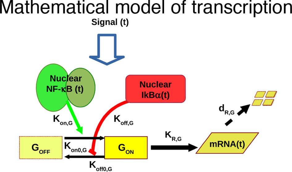
Mathematical model based on ODEs to fit single genes transcription; parameter names are reported.
https://doi.org/10.7554/eLife.09100.035
Figure 5—figure supplement 2

Hoechst staining does not affect transcription.
Quantitative PCR for nascent (left) and mature (right) IκBα (upper panels) and Ccl5 (bottom panels) in GFP-p65 MEFs cultured in 10% FCS or 0.1% FCS plus Hoechst. The cells were stimulated with TNF-α for the indicated times. The plots represent the average of two independent experiments. Bars: SEM.
Figure 6 with 7 supplements
Synchronized NF-κB dynamics translates into functionally different dynamical patterns of gene expression, each corresponding to distinct pathways.
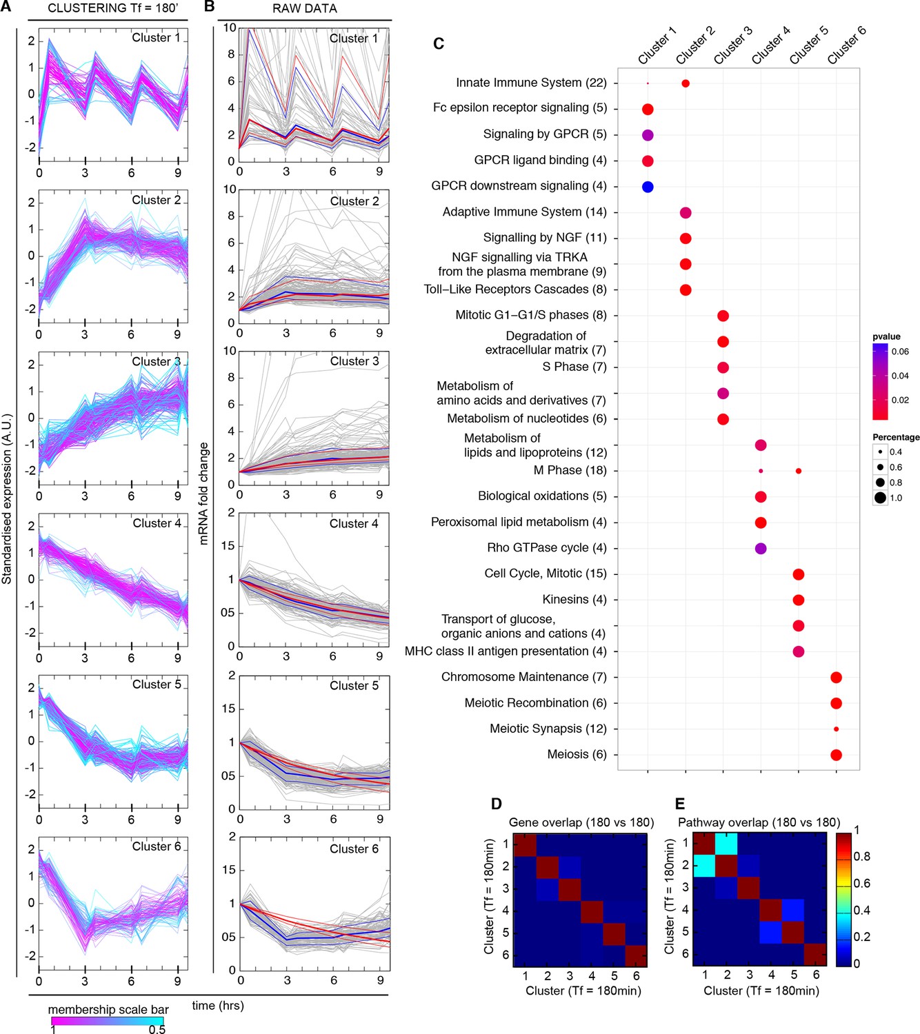
(A) Clusters 1–6 were obtained by an unsupervised k-means-like clustering from the genome-wide transcription profiling of samples harvested in the experiment shown in Figure 5A. Line colours are indicative of the membership value of each gene (colour scale at the bottom). Three clusters contain genes with increasing expression (1–3) and three with decreasing expression (4–6). On the y-axis, standardized expression profile in arbitrary units (see Materials and methods). (B) Plots show single-gene mRNA traces (median: thick blue line; 85% and 15% intervals, thin blue lines). The time courses can also be fitted using our minimal mathematical model: shown is the median of the single-gene fits (thick red line) and the 85% and 15% intervals (thin red lines). Fittings were performed using the same parameters for the external signal (PS) and the dynamics (PNF-κB) as in Figure 5, but using different gene expression parameters PG for each gene. (C) Top five pathways of hierarchical level 2 and 3 in the Reactome database significantly enriched in each dynamical cluster. Dot sizes are proportional to the percentage of genes in the cluster belonging to that pathway. Dot colours identify the corresponding p-values (p-value < 0.05 is set as threshold). Scale bars on the right. (D, E) Heatmaps shows the degree of overlap at gene level (D) and pathway level (E) between each of the 6 clusters. Colour scale bar on the right. Figure supplements from 1 to 6 are provided.
Figure 6—figure supplement 1
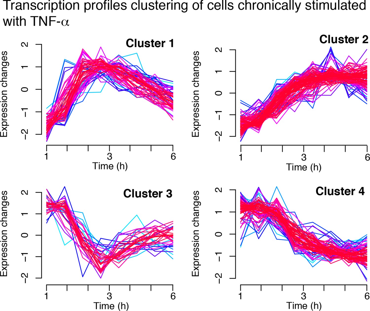
Transcription in cells chronically stimulated with TNF-α.
Four clusters are obtained from the standardized gene expression profiles for cells stimulated with a constant concentration of 10 ng/ml TNF-α. Each line represents a gene. Lines colors: blue and red indicate low and high membership values, respectively.
Figure 6—figure supplement 2
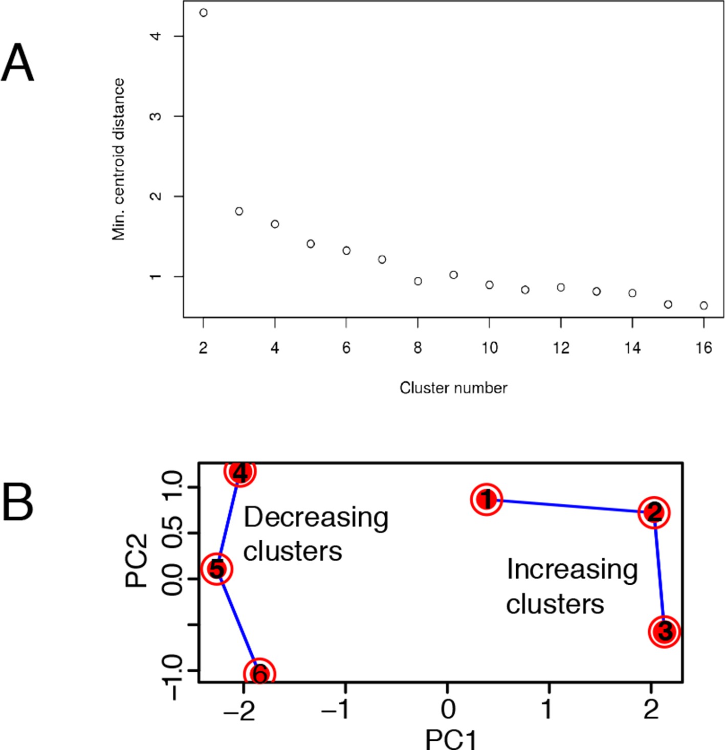
Mathematical validation of clustering.
(A) Minimal inter-centroid distance as a function of the number of clusters considered for Figure 6 . (B) Principal Component Analysis based on two components segregates clusters containing genes with increased transcription (1, 2 and 3) from those with decreased transcription (4, 5 and 6).
Figure 6—figure supplement 3
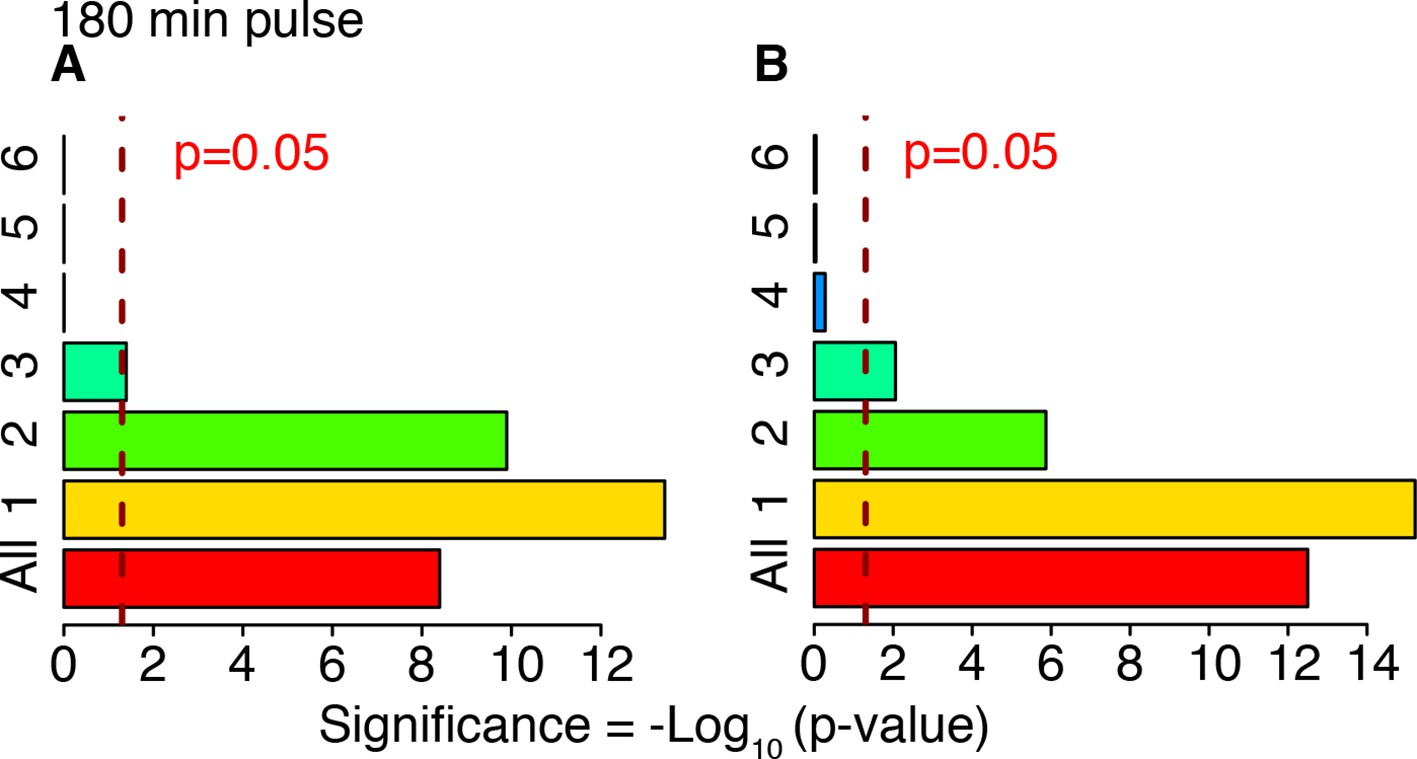
Cluster enrichment analysis for NF-κB targets in genes clustered and displayed in Figure 6.
Tf=180 with T1=30 min and T2=150 min. Two lists of NF-κB targets were considered. (A) Gilmore’s web-site (www.bu.edu/nf-kb/), (B) from (Li et al., 2014). Significance is shown as -Log10(p-value), a dashed line marks the threshold of significance at p=0.05.
Figure 6—figure supplement 4
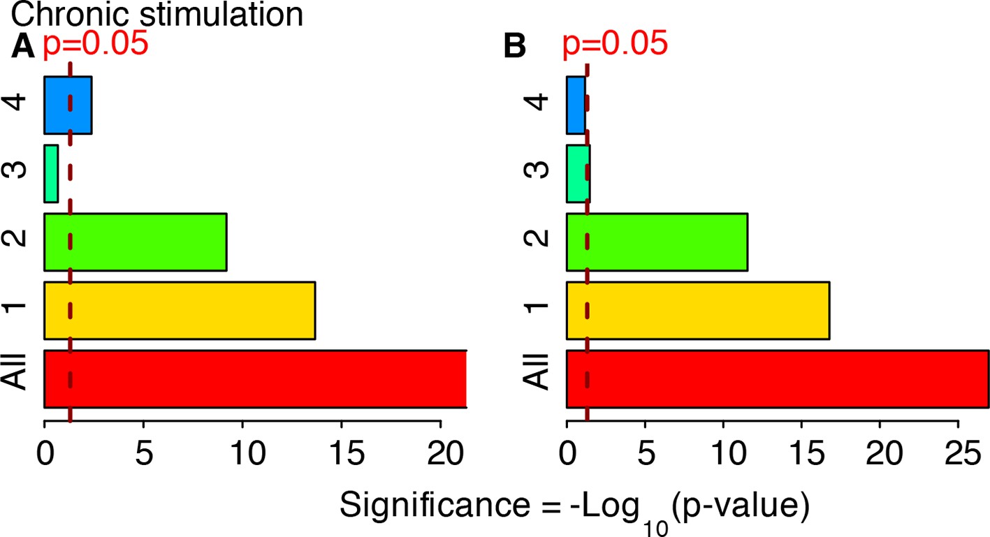
Cluster enrichment analysis for NF-κB targets in genes clustered and displayed in Figure 7 (constant stimulation).
Two lists of NF-κB targets were considered: (A) Gilmore’s web-site (www.bu.edu/nf-kb/). (B) from (Li et al., 2014). Significance is shown as –Log10(p-value), a dashed line marks the threshold of significance at p=0.05.
Figure 6—figure supplement 5

Distribution of fitting distances.
Distance distribution for single-gene fittings of genes with increased (left) or decreased (right) transcription in cells stimulated with a period of 180 min.
Figure 6—figure supplement 6
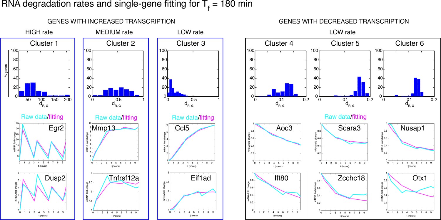
Degradation rates values are the key parameter to reproduce different gene expression patterns.
Upper panels: RNA degradation rates inferred from our model for the gene clusters, for a period of 180 min. Lower panels: example fittings of two genes for each cluster. Of note, the degradation rate is very high for oscillating genes in Cluster 1. Clusters 2 and 3 containing genes with “rapidly-increasing and slowly-decreasing” transcription or “slowly-increasing” transcription are characterised by degradation rates two orders of magnitude lower. Genes with decreasing transcription and belonging to Clusters 4–6 have very low RNA degradation rates.
Figure 6—figure supplement 7
Fitting of transcription data from the 180 min synchronization experiment with an alternative model of transcription.
The data were also fitted using a model in which IκBα (A) does not act as a transcriptional repressor in the feedbacks nor (B) in the expression of each single gene, while the role of NF-κB as transcriptional activator (green arrows in (A)) is preserved. (C) Gene expression data from the experiment in Figure 6 were fitted using the models of (A) and (B) analogously to our fittings of Figures 5 and 6 : with a common set of PNF-κB while each gene is fitted with its own PG. Again, the average relative error is lower for up-regulated genes. (D) Plots show single-gene traces (grey) of all mRNA (median: thick blue line; 85% and 15% intervals, thin blue lines). We show the median of the single-gene fits (thick red line) and the 85% and 15% intervals (thin red lines). (E) Histograms on the bottom part show the distribution of the degradation rates obtained from the fitting for each dynamical cluster. Here, again we have that the degradation rate is the key parameter to reproduce the gene expression patterns observed.
Figure 7 with 1 supplement
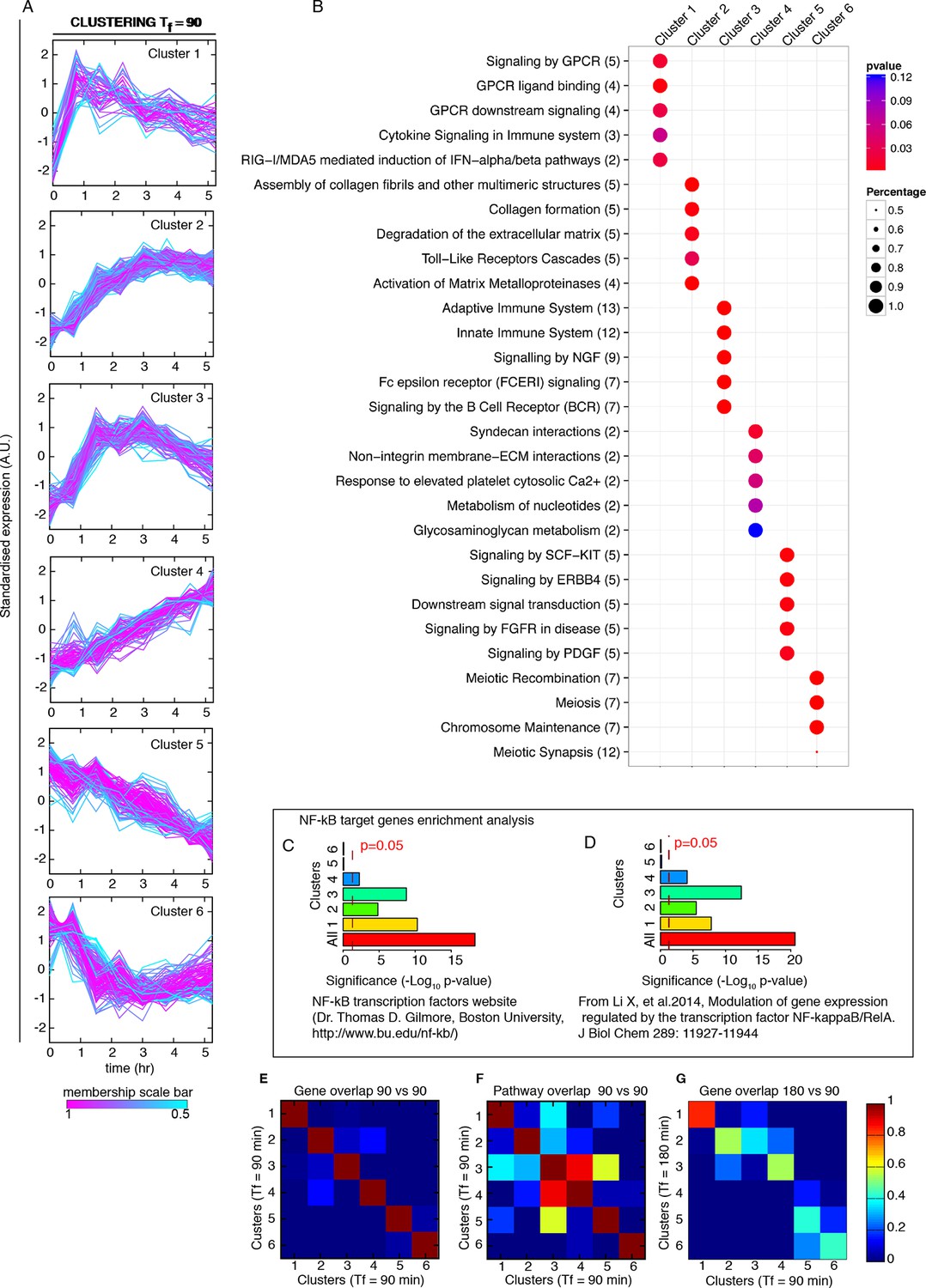
Genome-wide clustering for Tf=90 min.
(A) Clusters obtained by unsupervised k-means clustering from the genome-wide transcription profiling of cells perturbed with a forcing of 90 min, D1=10 and D2=0 ng/ml of TNF-α. Lines colours: blue and red indicate low and high membership values, respectively. (B) Top five pathways of hierarchical level 2 and 3 in the Reactome database significantly enriched in each dynamical cluster. Dot sizes are proportional to the percentage of genes in the cluster belonging to that pathway. Dot colours identify the corresponding p-values (p-value<0.05 is set as threshold). Scale bars on the right. (C, D) Enrichment analysis for NF-κB targets from the clusters displayed in panel A. Two lists of NF-κB targets were considered: left: Gilmore’s web-site (www.bu.edu/nf-kb/); right: data from Brasier and Kudlicki groups (Li et al., 2014). Significance is shown as -Log(p-value), a dashed line marks the threshold of significance at p=0.05. (E, F) Heatmaps show the degree of overlap at gene level (E) and pathway level (F) between each of the 6 clusters. (G) Overlap at a gene level between clusters obtained for 180 min and for 90 min. It is particularly high for Clusters 1, those of oscillating genes. Colour scale bar on the right. Figure supplement 1 is provided.
Figure 7—figure supplement 1
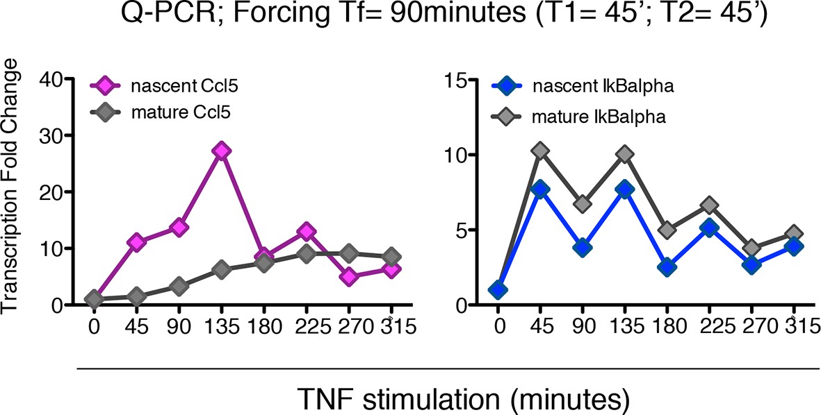
Synchronous NF-κB oscillations arising with 90 min forcing lead to population-level coordinated transcription.
Q-PCR time-course of nascent and mature mRNAs for the prototypical late and early genes Ccl5 and IκBα are shown. PCR assays were performed on the same samples used for genome-wide transcription profiling shown in Figure 7.
Figure 8
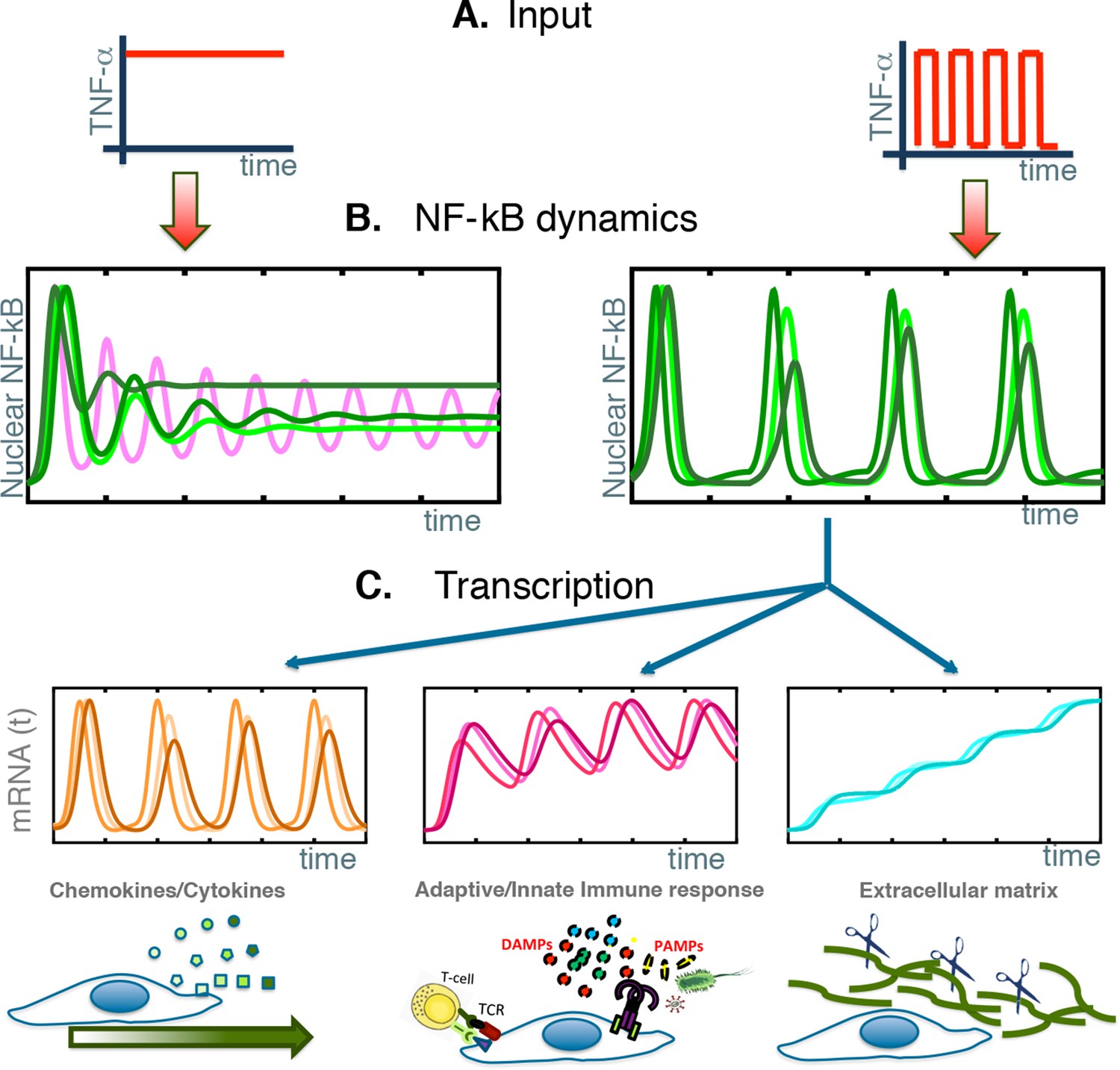
NF-κB behaves as a damped oscillator that can synchronize to time-varying external stimuli to produce functionally related transcriptional outputs.
(A) The NF-κB system is able to provide different responses to different inputs, from constant (left) to time-varying ones (right). (B) Our cells show damped oscillations to a constant stimulus (left, green lines), although for other cell types sustained oscillations might be possible (magenta line). Damped oscillations can adapt to timevarying inputs (right) and give rise to synchronous oscillations. (C) These synchronous oscillations produce different patterns of gene expression, from oscillating (left, orange lines) to slowly increasing (right, blue lines) and intermediate dynamics (pink lines, centre). We find that each kind of dynamics is typical for genes involved in different cellular functions.
Videos
Video 1
Dynamics for constant flow of TNF-α.
Imaging of GFP-p65 knock-in cells in the microfluidic chamber stimulated with a constant flow of 10 ng/ml TNF-α for 12 hr. The stimulus induced nuclear-to-cytoplasmic p65 oscillations that are qualitatively similar to the heterogeneous oscillations observed with static stimulation. Along time, it is possible to appreciate the increase of TNF-induced cell death and apoptosis.
Video 2
Dynamics for Hoechst-stained cells in the absence of TNF-α.
Several controls were performed to exclude possible damaging effects related to imaging. This video shows that cells under constant flow of fresh medium without TNF-α divide and very few events of cell death are detectable. Left part: GFP channel; right part HOE channel. Twelve-hour imaging.
Video 3
Dynamics for Tf=90 min.
Imaging of cells stimulated with D1 =10 ng/ml TNF-α, D2 =0 ng/ml and Tf=90 min. (T1=45 min and T2 =45). Peaks are present in all the forcing cycles and synchronous. Twelve-hour imaging.
Video 4
Dynamics for Tf=180 min.
Imaging of cells stimulated with D1 =10 ng/ml TNF-α, D2 =0 ng/ml and Tf=2T0=180 min (T1=30 min and T2 =150). Oscillations are locked to the forcing. Twelve-hour imaging.
Video 5
Dynamics for Tf=45 min.
Imaging of cells stimulated with D1 =10 ng/ml TNF-α, D2 =0 ng/ml and Tf=T0/2=45 min (T1=22.5 min and T2 =22.5 min). Such short wash-out provides a sufficient resetting of the external signal; in these conditions we obtained a sharply defined dynamical response and oscillations are locked in step. Twelve-hour imaging.
Video 6
Dynamics for Tf=60 min.
GFP-p65 cells can be synchronized under periodic stimulations with Tf=60 min (T1 =T2 =30 min) when D1 =10 ng/ml and D2 =0 ng/ml. Twelve-hour imaging.
Additional files
-
Supplementary file 1
RT-PCR primers list.
Listed are the primers used in Q-PCR reaction to test gene expression as reported in Figure 5 and in Figure 5—figure supplement 2 and Figure 7—figure supplement 1.
- https://doi.org/10.7554/eLife.09100.048
-
Supplementary file 2
Biochemical rates for the model.
In this file we indicate the biochemical rates and the constants considered, which are described in the Materials and methods. We also provide the value of these rates and the bibliographic reference from which they were taken, if any. Otherwise, we motivate our selection of the value or we state that they were manually fitted. We also indicate the related model parameters resulting from the adimensionalization of the equations of the dynamics and the uncertainty degree, a measure of how uncertain each parameter value is. This is also a measure of how much we allow each parameter to vary in our exploration of the dynamics of the system and in our fittings. Notice that higher uncertainty degrees are assigned to parameters that were manually fitted or to those that are involved in reactions from our models that summarize many different biochemical processes.
- https://doi.org/10.7554/eLife.09100.049
Download links
A two-part list of links to download the article, or parts of the article, in various formats.
Downloads (link to download the article as PDF)
Open citations (links to open the citations from this article in various online reference manager services)
Cite this article (links to download the citations from this article in formats compatible with various reference manager tools)
NF-κB oscillations translate into functionally related patterns of gene expression
eLife 5:e09100.
https://doi.org/10.7554/eLife.09100


