Nonlinear circuits for naturalistic visual motion estimation
- Harvard University, United States
- Yale University, United States
Figures
Figure 1
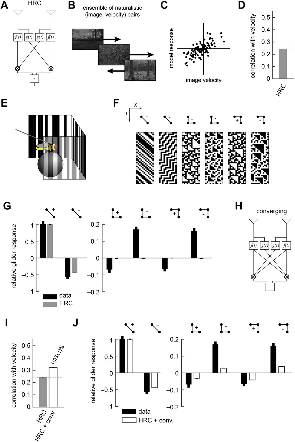
The Hassenstein-Reichardt correlator (HRC) model is an incomplete description of Drosophila's motion estimator.
(A) Diagram of the HRC model. (B) We assessed motion estimation performance across an ensemble of naturalistic motions, each of which consisted of a natural image (van Hateren and van der Schaaf, 1998) and a velocity chosen from a normal distribution. (C) We quantified model accuracy by comparing the model response to the true velocity using the mean squared error. (D) We summarized the error with the correlation coefficient between the model output and the true velocity. (E) In previous work (Clark et al., 2014), we used a panoramic display and spherical treadmill to measure the rotational responses of Drosophila to visual stimuli. (F) We presented flies with binary stimuli called gliders (Hu and Victor, 2010), which imposed specific 2-point and 3-point correlations (Clark et al., 2014). (G) Flies turned in response to 3-point glider stimuli, but these responses cannot be predicted by the standard HRC. (H) Diagram of the converging 3-point correlator, which is designed to detect higher-order motion signals like those found in 3-point glider stimuli. (I) Adding the converging 3-point correlator to the HRC improved motion estimation performance with naturalistic inputs. We optimized weighting coefficients to minimize the mean squared error over the ensemble of naturalistic motions and used cross-validation to protect against over-fitting. (J) This model predicted that Drosophila would weakly turn in response to 3-point glider stimuli.
Figure 2 with 1 supplement
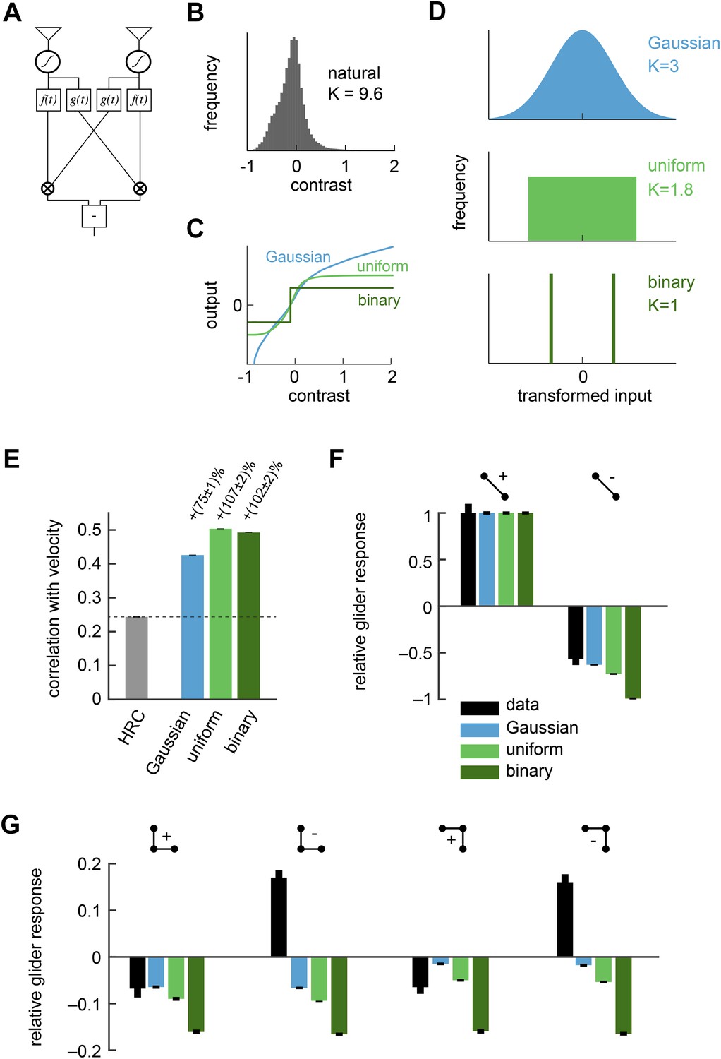
Front-end nonlinearities improved naturalistic motion estimation but did not reproduce the psychophysical results.
(A) Diagram of the front-end nonlinearity model. The nonlinearity occurs after the spatiotemporal filtering of photoreceptors but before the temporal filtering of the HRC. (B) The distribution of contrast signals after photoreceptor filtering had a kurtosis of 9.6. The kurtosis of unfiltered pixels in the image database was 7.8. (C) Three different nonlinearities that transformed this input distribution into a Gaussian distribution, a uniform distribution, and a binary distribution. (D) After these transformations, the kurtosis of the contrast signal was reduced to 3, 1.8, and 1, respectively. (E) Each front-end nonlinearity model improved the HRC's estimation accuracy, and uniform output signals worked best. (F, G) The front-end nonlinearity models reproduced the sign of the negative 2-point glider psychophysical responses but did not reproduce the pattern of psychophysical responses to 3-point gliders.
Figure 2—figure supplement 1
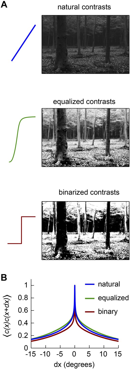
Front-end nonlinearities modify the correlations present in natural scenes.
(A) Example images with no front-end nonlinearity (top), with an equalizing front-end nonlinearity (middle), and with a binarizing front-end nonlinearity (bottom). (B) The covariance between contrasts at 2 horizontally separated points is plotted as a function of distance between the points. The binary nonlinearity attenuated spatial correlations.
Figure 3 with 2 supplements
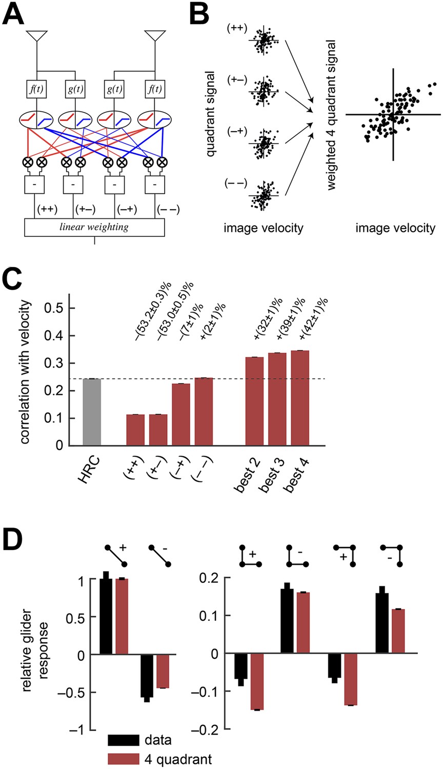
The weighted 4-quadrant model improved estimation performance and reproduced the directionality of psychophysical results.
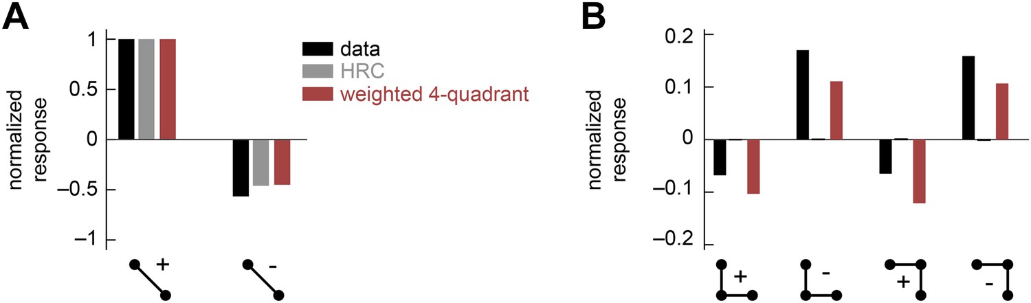
(A) Diagram of the weighted 4-quadrant model. Similar to ON/OFF processing in the visual system, the weighted 4-quadrant model splits the four differentially filtered signals into positive and negative components. As in the HRC, these component signals are paired, multiplied, and subtracted to produce four mirror anti-symmetric signals. We refer to these signals as HRC-quadrants. The model output is a weighted sum of the quadrant signals. We identify quadrants by whether they respond to the positive or negative components of each filtered signal and denote the four quadrants as (+ +), (+ −), (− +), and (− −). In this notation, the first index refers to the sign of the low-pass filtered signal (emanating from ), and the second refers to the high-pass filtered signal (emanating from ). (B) We measured the response of each quadrant to naturalistic motions and chose the quadrant weightings to minimize the mean squared error between the model output and the true velocity. (C) Comparison of the estimation performance of individual quadrants, multiple quadrants, and the HRC. The best two quadrants were (− −) and (− +); the best three also included (+ −). (D) The performance-optimized weighted 4-quadrant model reproduced the signs and approximate magnitudes of the psychophysical results.
Figure 3—figure supplement 1
Separate ON and OFF processing improved motion estimation by supplementing the HRC with odd-ordered correlations.
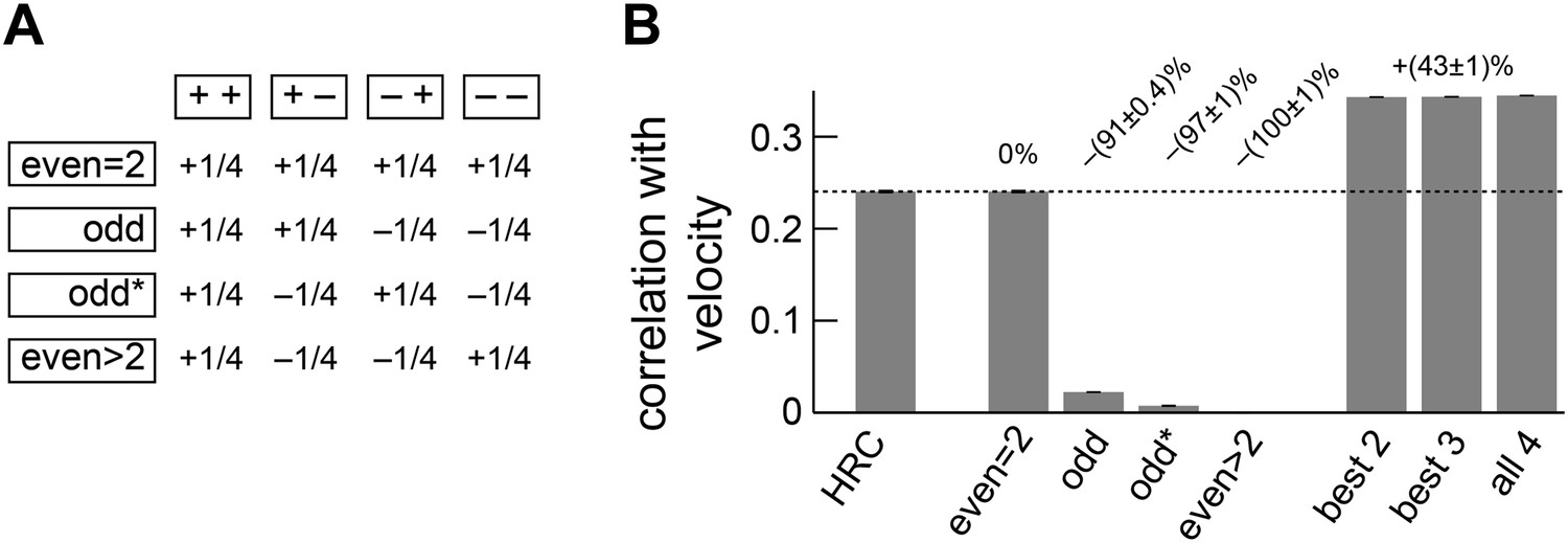
(A) By summing and subtracting the four quadrants (top labels, e.g., ‘++’) in four different patterns, we isolated the contributions of various correlation types (side labels, e.g., ‘odd’) to the weighted 4-quadrant model (Appendix 7). For example, the uniform sum of the four quadrants is the HRC, and we denote this quadrant combination as ‘even = 2’ (top row of matrix). The other three rows of the matrix define quadrant combinations that are sensitive to two different classes of third and higher odd-ordered correlations (‘odd’ and ‘odd*’ rows) and to fourth and higher even-ordered correlations (‘even >2’ row). The factor of 1/4 merely sets the magnitude of the quadrant contributions to match the formulas in Appendix 7 and is without conceptual importance. (B) The ‘even = 2’ correlation class worked best in isolation. Nevertheless, the ‘even = 2’ and ‘odd’ classes were highly synergistic (their weighted sum is notated ‘best 2’), and these classes together made the ‘odd*’ and the ‘even >2’ classes irrelevant.
Figure 3—figure supplement 2
The weighted 4-quadrant model cannot reproduce the positive-negative parity asymmetry in the psychophysical data.
In this numerical experiment, we tuned the coefficients of the weighted 4-quadrant model to optimize a fit to the psychophysical data. (A) The tuned model could reproduce the 2-point glider data well. (B) Although the tuned weighted 4-quadrant model could reproduce the signs of the 3-point glider data, it could not reproduce the differential amplitudes of the positive and negative parity responses. This demonstrates that the architecture of the weighted 4-quadrant model is too limited to reproduce the experimental response pattern.
Figure 4 with 2 supplements

Several biologically motivated generalizations of the motion estimator further improved estimation performance without sacrificing glider responses.
See Table 1 for a description of the biological rationales behind these models. (A) The ‘non-multiplicative nonlinearity’ model substitutes a 2-dimensional nonlinearity for the pure multiplication of the HRC. Here, we approximated the nonlinearity with a fourth order polynomial. (B) Two-dimensional nonlinearities underlying the HRC, the weighted 4-quadrant model, and the non-multiplicative nonlinearity model. The latter models reflect optimized cases, in which the weighting coefficients maximized estimation performance with natural inputs. Iso-output lines are shown in each plot, and the horizontal and vertical limits are chosen to include 95% of the naturalistic input signals. (C) Another generalization, the ‘unrestricted nonlinearity’ model allows all 4 input signals to be combined nonlinearly. We approximate this 4-dimensional nonlinearity with a fourth-order polynomial. (D) A final generalization, the ‘extra input nonlinearity’ model, relaxes the restriction that the motion estimator only uses 2 spatial inputs. We approximate this 6-dimensional nonlinearity with a fourth-order polynomial. (E) Comparison of the estimation performance of these models to the HRC. We compare the extra input nonlinearity model to the average of two neighboring motion estimators. (F, G) The three models correctly predicted the directions of psychophysical responses. The pattern of 3-point responses differed somewhat across the models, and the extra input nonlinearity model was the first to predict a large asymmetry between positive and negative 3-point glider responses.
Figure 4—figure supplement 1
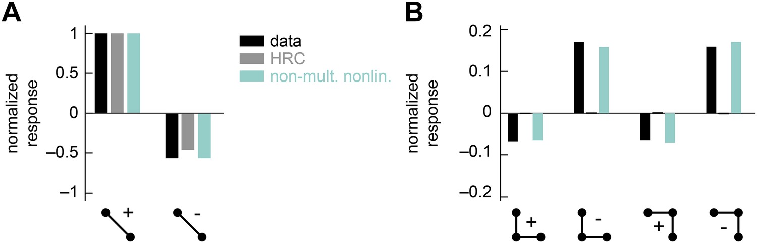
The non-multiplicative nonlinearity model can be tuned to account for the positive-negative parity asymmetry in the psychophysical data.
In this numerical experiment, we tuned the model nonlinearity to optimize a fit to the psychophysical data. (A) In this case, the tuned model could reproduce the 2-point glider data well. (B) This tuned model could also reproduce the differential amplitudes of the positive and negative parity responses. Thus, the non-multiplicative nonlinearity model repairs an architectural defect of the weighted 4-quadrant model (Figure 3—figure supplement 2).
Figure 4—figure supplement 2
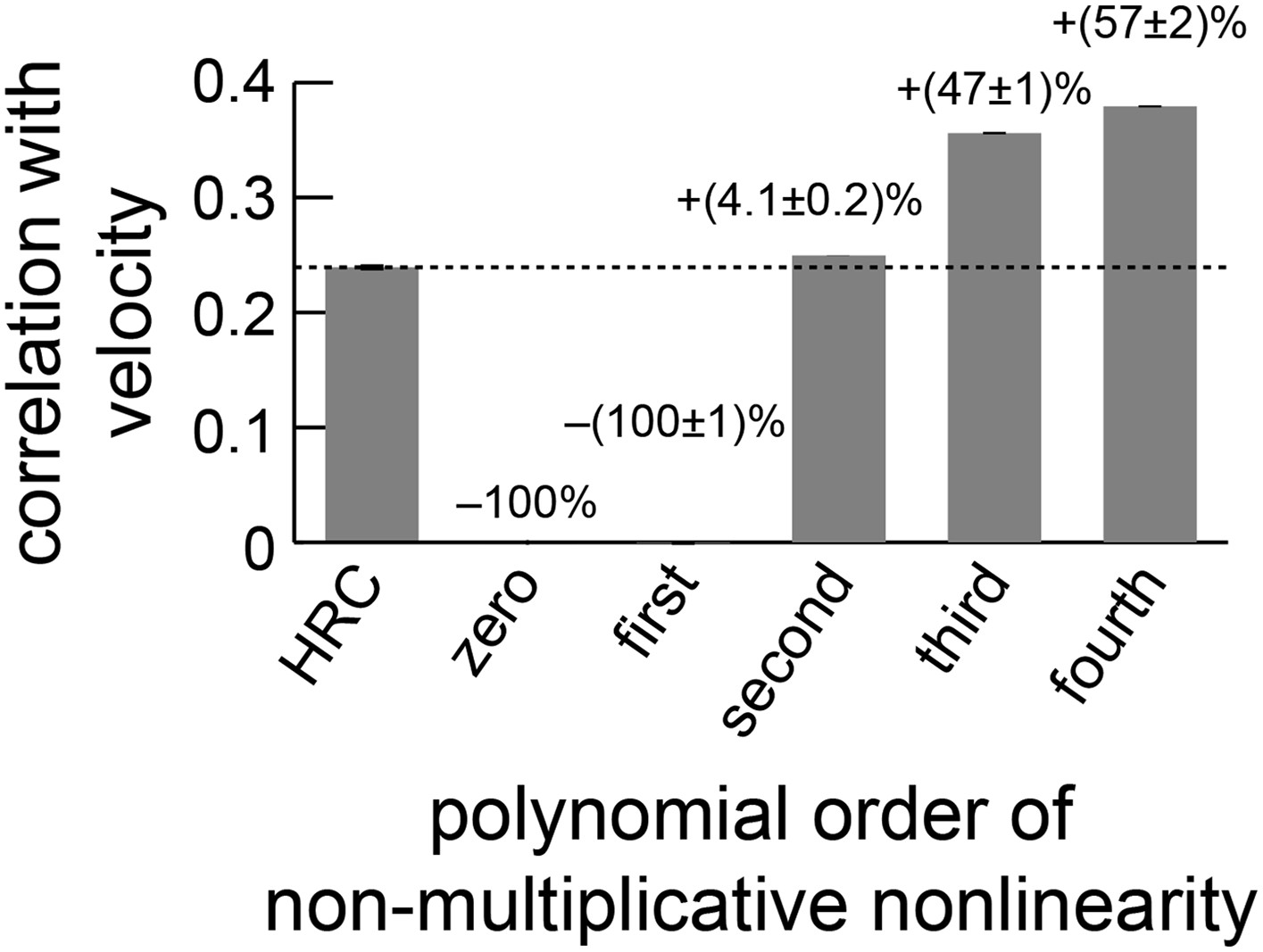
The performance of the non-multiplicative nonlinearity model is plotted against the order of the fitted polynomial.
With only zeroth or first-order terms, the model cannot predict motion. With second-order terms, it can perform slightly better than the HRC (Appendix 10). The biggest performance increase occurred when third-order terms were included, and the fourth-order terms also improved performance.
Figure 5 with 1 supplement

Computational interpretation of the extra input nonlinearity model.
(A) We used lasso regression to select subsets of predictors that might enable accurate estimation (see ‘Materials and methods’). With only 16 predictors, the model improved naturalistic performance over the HRC by 68%, and including fewer than half of the predictors improved it by the full 92%. The maximum number of predictors corresponds to the number of polynomial coefficients that were fit in the full model. (B) We visualized the 6-dimensional nonlinearity as the sum of several simpler computational modules. When only 16 predictors were used (red bar in (A)), the model used four distinct types of computations. In particular, the model included nearest-neighbor and next-nearest-neighbor non-multiplicative nonlinearities (top row). It also included a converging 3-point correlator from the two furthest photoreceptors and a 4-point correlator that combined three spatial inputs (bottom row). (C) Venn diagram illustrating the hierarchical nesting of models used in this paper. All models in this paper contain sets of parameters that reproduce the HRC (gray dot). The weighted 4-quadrant model is a subset of non-multiplicative nonlinearity models, which are themselves a subset of unrestricted nonlinearity models. The extra input nonlinearity encompasses all the models. When we approximated the nonlinearites with fourth order polynomials, we restricted them to a smaller portion of the model space. The 4-quadrant nonlinearities only overlapped with the fourth-order polynomial approximation at the HRC, because the weighted 4-quadrant model is infinite order when expanded as a polynomial (see Appendix 7).
Figure 5—figure supplement 1
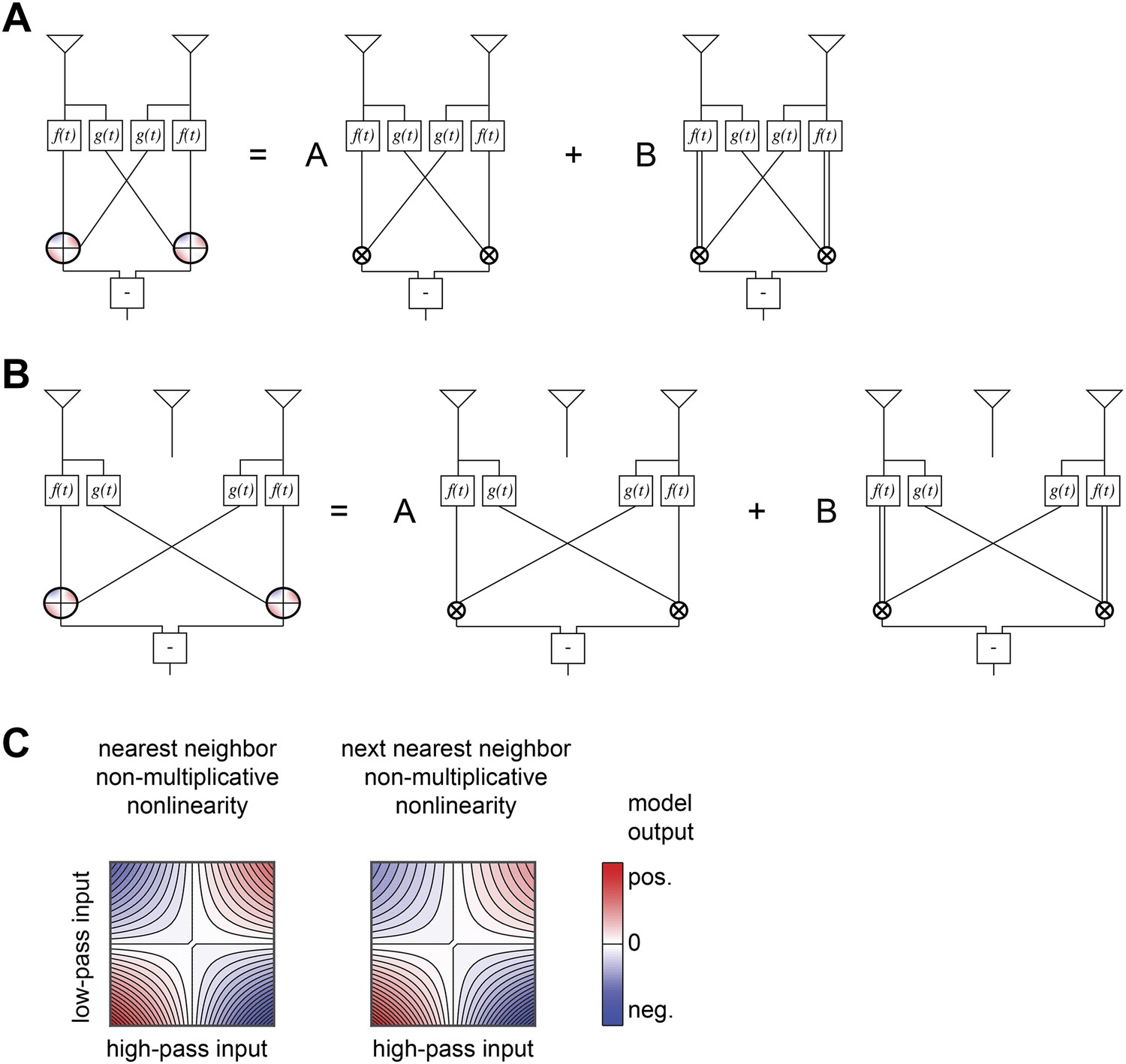
Structure of non-multiplicative nonlinearities in the extra input model of Figure 5B.
(A) The nearest-neighbor non-multiplicative nonlinearity was made up of a standard HRC and a 3-point correlator in which the low-pass filtered input was squared before being multiplied by the adjacent receptor's high-pass filtered signal. (B) The next-nearest-neighbor non-multiplicative nonlinearity combined the analogous long-range terms. (C) Structure of the 2-dimensional nonlinearities, shown according to the same conventions as Figure 4B.
Appendix figure 1

Motion transforms spatial correlations into temporal correlations.
(A) An example natural image (van Hateren and van der Schaaf, 1998). (B) When a natural image (top face) moves to the right, streaks in space-time (front face) indicate the direction and speed of the motion. Alternatively, motion influences the temporal correlation structure of visual signals (side face). (C) Second-order correlation function between pairs of spatially separated contrast signals (across the natural image ensemble [van Hateren and van der Schaaf, 1998]). (D) For constant velocity motion, the temporal correlation function between a pair of spatially separated points is shifted and stretched relative to the spatial correlation function. We separated the two points by Drosophila's photoreceptor spacing (5.1°). (E) Example third-order spatial correlation function involving two points in space. (F) As with pairwise correlations, higher-order temporal correlations between spatially separated visual signals are shifted and stretched (relative to higher-order spatial correlation functions) in a manner that indicates the speed and direction of motion.
Appendix figure 2

Correlations in binarized natural images.
(A) We transformed each image in the van Hateren natural image database (van Hateren and van der Schaaf, 1998) with several binarizing nonlinearities. To implement the simplest binarizing nonlinearity, we set all pixels to +1 or −1 depending on whether that pixel exceeded or fell below the median intensity in the image. For the nonlinearity with two steps, the thresholds were at the 25th and 75th intensity percentiles. For the nonlinearity with three steps, the thresholds were at the 25th, 50th, and 75th intensity percentiles. When a pixel intensity exactly equaled a threshold, we considered its value below threshold. Binary nonlinearities with a larger number of steps produced grainier images that indicate a spatial decorrelation of the transformed image. (B) We computed second-order spatial correlation functions across the nonlinearly transformed natural image ensemble. This confirmed that each step in the binarizing nonlinearity further decorrelated the image ensemble. (C) In addition to decreasing the spatial extent of correlations, a larger number of transitions also degraded the performance of the front-end nonlinearity model.
Appendix figure 3
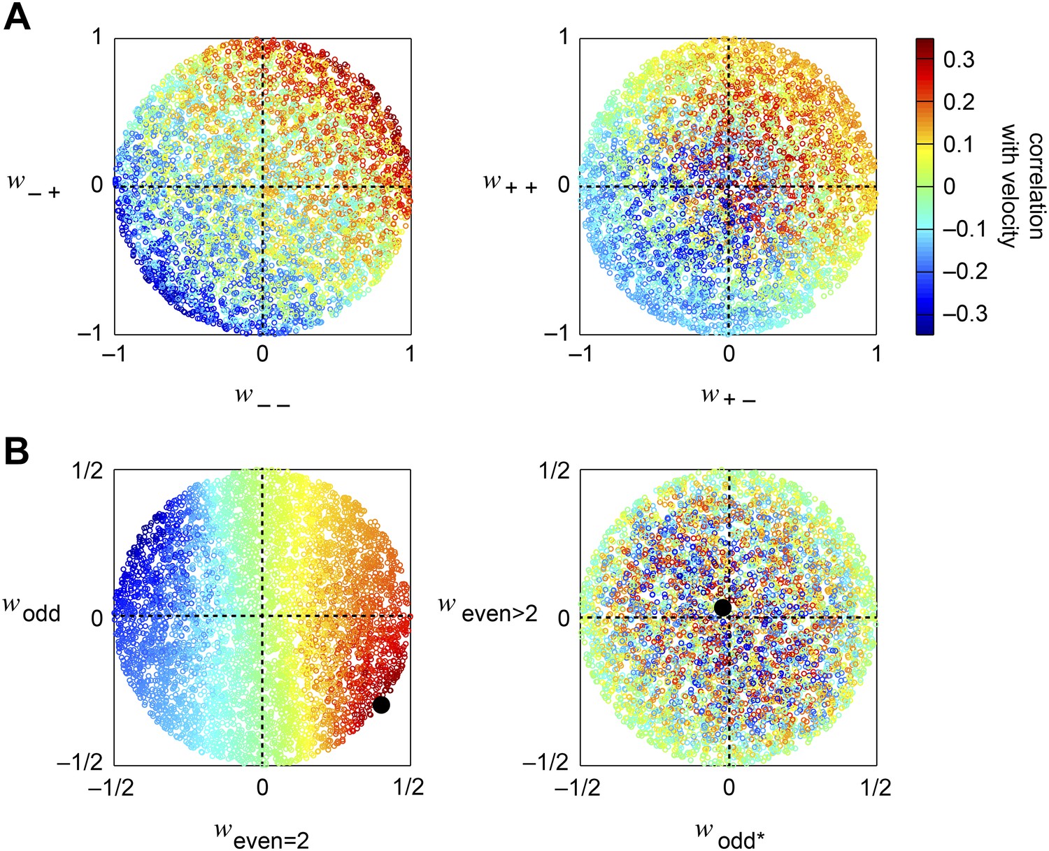
Accuracy of the weighted 4-quadrant model across model parameters.
(A, B) We computed the correlation coefficient between the velocity and the response of the weighted 4-quadrant model for all possible sets of model parameters. Since rescaling the weight vector does not affect the correlation coefficient, we assumed that all model parameters satisfy . We color-coded each set of model parameters by its accuracy and projected the parameter space onto various subspaces. (A) We first examined the quadrant basis by projecting onto the {(− −), (− +)} (left) and {(+ −), (+ +)} (right) subspaces. (B) We next examined the correlational basis by projecting onto the {even = 2, odd} (left) and {odd*, even >2} (right) subspaces. These project into different linear combinations of the original quadrant weightings. One of the projections is the pure HRC (even = 2), while the other projections contain only odd correlations, of two different types (odd and odd*), or only even correlations of order greater than 2 (even >2). These projections show that accurate weighted 4-quadrant models always put positive weight into 2-point correlations and negative weight into odd-ordered correlations. Note that the glider responses predicted by the weighted 4-quadrant model mirror this pattern (Figure 3D).
Appendix figure 4
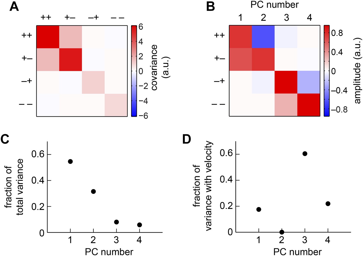
The weighted 4-quadrant model in the basis of principal components (PCs).
(A) We computed the covariance matrix of quadrant responses across the simulated ensemble of naturalistic motions. (B) The eigenvectors of the covariance matrix are called PCs. Signals from the (+ +) and (+ −) quadrants primarily comprised the first two PCs, whereas the (− +) and (− −) components comprised the third and fourth PCs. (C) The first two PCs accounted for the vast majority of the weighted 4-quadrant model's response variance. (D) Each member of the ensemble of naturalistic motions comprised a velocity and a natural image, and both components contributed variance to the model response. Although the first two PCs accounted for most of the variance, little of that variance was associated with the velocity of motion. Instead, the third and fourth PCs best aided motion estimation, because they contributed the vast majority of the velocity-associated variance.
Tables
Table 1
The different models used in this paper, experimental results that support each model, and references for those results
| Model | Supporting evidence |
|---|---|
| Front-end nonlinearity | • Photoreceptors show nonlinear responses to contrast changes (Laughlin, 1989; Juusola and Hardie, 2001; Juusola and Hardie, 2001; van Hateren and Snippe, 2006) |
| • Some neurons in the early visual system have nonlinear responses that make their output signals nearly uniform (Laughlin, 1981) | |
| Weighted 4-quadrant model | • Visual processing is divided early into ON and OFF channels (Joesch et al., 2010; Clark et al., 2011; Behnia et al., 2014; Meier et al., 2014; Strother et al., 2014) |
| • The two output channels (T4/T5) are sensitive to light and dark edges (Maisak et al., 2013), but their inputs are incompletely rectified (Behnia et al., 2014) | |
| • Stimuli targeting the four quadrants are differentially represented in neural substrates (Clark et al., 2011; Joesch et al., 2013) | |
| Non-multiplicative nonlinearity | • Pure multiplication is not a trivial neural operation (Koch, 2004) |
| • Inputs to T4/T5 are nonlinearly transformed (Behnia et al., 2014), which also contributes to the biologically implemented non-multiplicative nonlinearity | |
| Unrestricted nonlinearity | • The direction-selective neurons T4 receive inputs from more than two types of neurons (Takemura et al., 2013; Ammer et al., 2015) |
| • T4 receives inputs from both its major input channels at overlapping points in space (Takemura et al., 2013) | |
| Extra input nonlinearity | • The direction-selective neuron T4 receives inputs from more than two discrete retinotopic locations (Takemura et al., 2013) |
Additional files
-
Source code 1
Code used to generate figures.
- https://doi.org/10.7554/eLife.09123.021
Download links
A two-part list of links to download the article, or parts of the article, in various formats.
Downloads (link to download the article as PDF)
Open citations (links to open the citations from this article in various online reference manager services)
Cite this article (links to download the citations from this article in formats compatible with various reference manager tools)
Nonlinear circuits for naturalistic visual motion estimation
eLife 4:e09123.
https://doi.org/10.7554/eLife.09123


