Using an achiasmic human visual system to quantify the relationship between the fMRI BOLD signal and neural response
- University of Southern California, United States
- University of California, Berkeley, United States
Figures
Figure 1 with 1 supplement
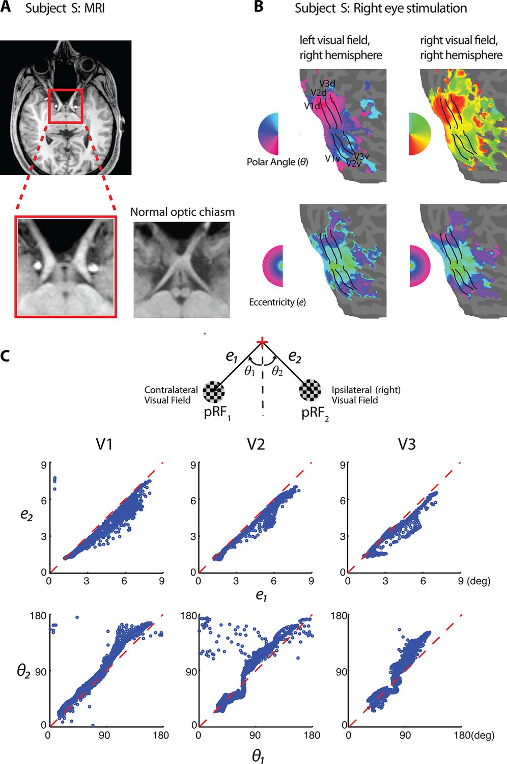
Retinotopy of the achiasmic subject S.
(A) The MRI image of S shows the lack of the optic chiasm. (B) S has a well-defined retinotopy, but unlike normal retinotopic representations, both left and right visual fields are mapped to the same hemisphere ipsilateral to the stimulated eye (data from right-eye stimulation are shown). Eccentricity and polar angle maps are organized orderly for both visual hemifields. Visual area boundaries were identified at where the polar angle reversed. (C) A schematic of the two population receptive fields (pRFs) of a fMRI voxel. For individual voxels in V1-V3, eccentricities (upper panels) and polar angles relative to the lower vertical meridian (lower panels) of each of the two pRFs are plotted against each other. Most values fall close to the identity line, demonstrating that the two pRFs of each voxel are at mirrored locations across the vertical meridian.
Figure 1—figure supplement 1
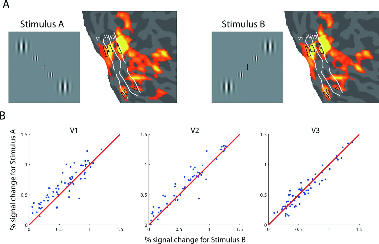
fMRI BOLD response evoked with ROI-defining stimuli.
(A) The ROI-defining stimuli in the backward-slash (Stimulus A) and forward-slash (Stimulus B) configurations. The corresponding areas with significant modulation (FDR<0.05) are depicted on the flattened visual cortex of the right hemisphere of the achiasmic subject, who viewed the stimuli with his right eye. These stimuli were used to define the ROIs for the analyses of the adaptation experiment (Figure 2) and the BOLD summation experiment (Figure 3). White lines delineate the borders of the retinotopically defined visual areas. Black contours outline the boundaries of the ROIs used in the experiments, corresponding to the middle 2 degrees (diameter) of the larger (4-degree diameter) outer Gabor patches. (B) BOLD response amplitudes of Stimulus A versus those of Stimulus B for randomly selected voxels in areas V1-V3. The stimuli evoked nearly identical responses in each voxel, suggesting that (1) each voxel has two pRFs and (2) the neural populations underlying each pRF are nearly identical.
Figure 2 with 1 supplement
Behavioral and physiological evidence of independence between the co-localized neural populations.
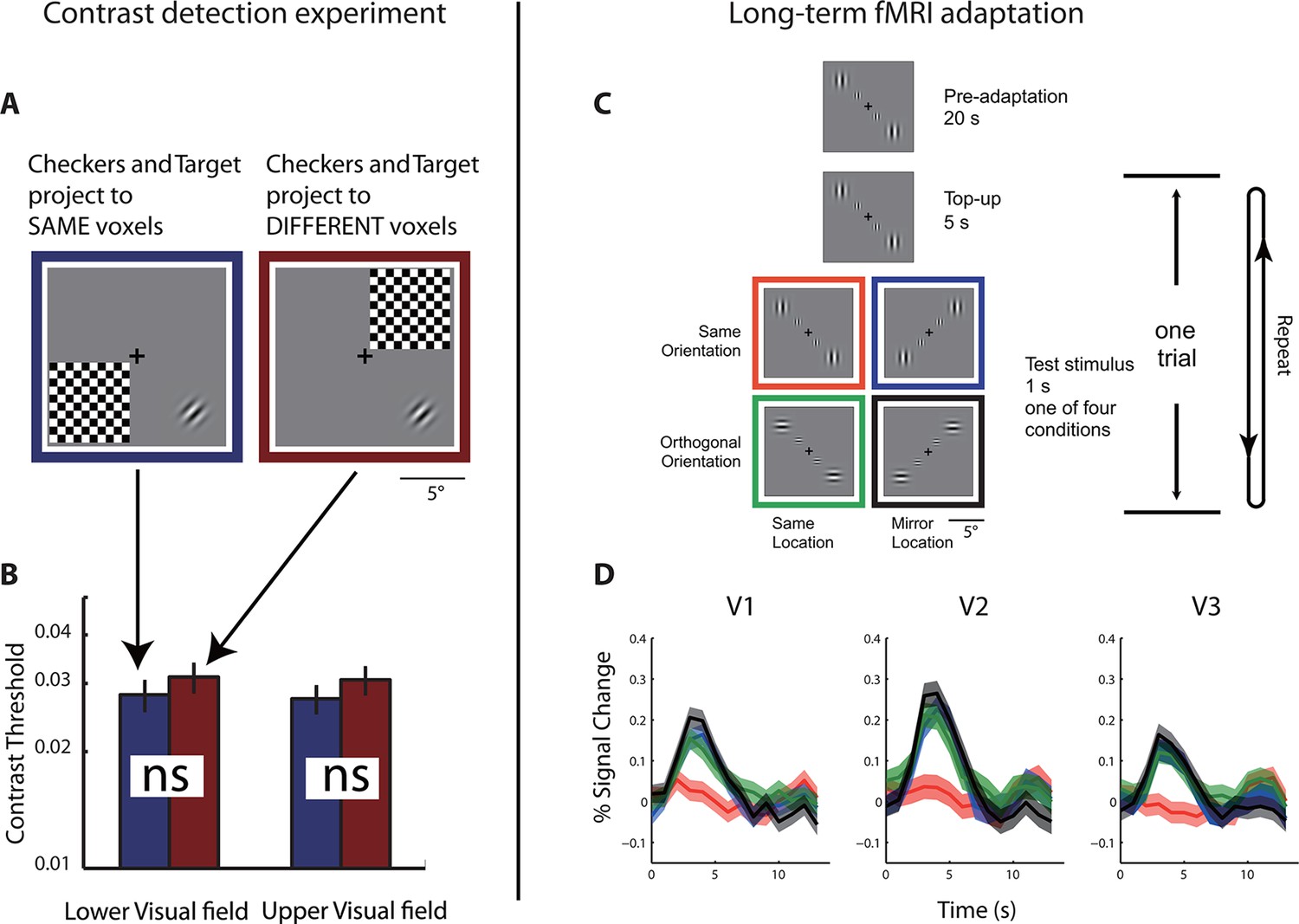
(A) Schematic of the psychophysical experiment of contrast detection with a contralateral mask. The 45° target Gabor patch was presented in either the lower-right (shown) or upper-left quadrant. A high-contrast flickering checkerboard mask was presented at the mirrored location from the target quadrant, across either the vertical or horizontal meridian. S was to identify which one of the two temporal intervals the target appeared in. (B) Contrast detection thresholds were essentially the same for the two mask-target arrangements. Error bars denote ± SE across blocks. (C) Design of the fMRI adaptation experiment. Each block of trials was preceded with 20 s of pre-adaptation. Each trial began with a 5 s presentation of the adapting stimulus (‘top-up’ adaptation), followed by one of the four test stimuli. Relative to the adapting stimulus, the test stimulus could either be at the same or mirrored location, and could have either the same or orthogonal orientation. Attention was controlled with a demanding central fixation task. (D) Time courses of fMRI BOLD responses in V1-V3 to the four test conditions. Shaded error band denote ± SE across trials. The responses evoked by the test stimuli presented at the mirrored location relative to the adaptor, regardless of orientation, did not differ significantly from those evoked by the test stimuli at the same location as the adaptor but with orthogonal orientation.
Figure 2—figure supplement 1
Results from supplementary psychophysical experiments implicating two groups of non-interacting neurons.
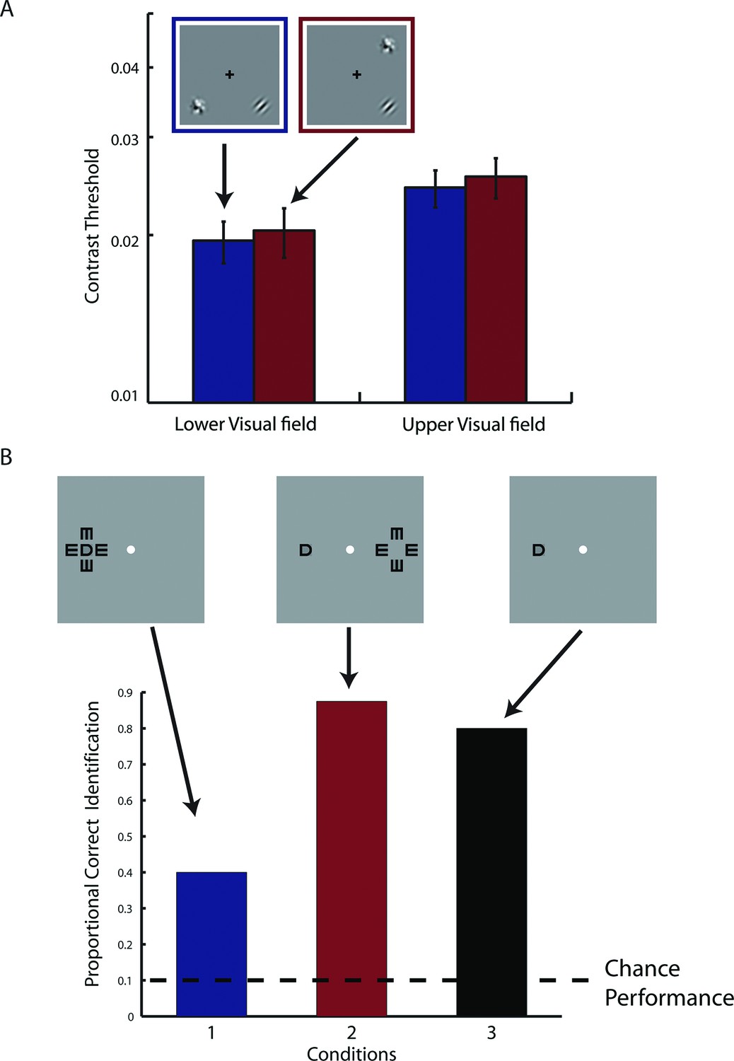
(A) Contrast detection task with a contralateral noise mask. The target Gabor patch was presented in either the lower-right (shown) or upper-left quadrant. An isotropic noise mask of the same spatial frequency band as the target was presented at the mirrored location of the target across either the vertical or horizontal meridian. In the cross-vertical-meridian arrangement (blue), but not in the cross-horizontal-meridian arrangement (red), both the target and the mask projected to the same cortical locations in V1-V3 of the achiasmic subject S. S was to identify which one of the two temporal intervals contained the target. Contrast detection thresholds were essentially identical for the two mask positions. Error bars denote ± SE across different blocks. (B) Letter identification task: S’s task was to identify the target (center) letter presented at an eccentricity of 10 deg and flanked with the 4 tumbling E’s. The target letter was randomly drawn from the set of 10 letters (C, D, H, K, N, O, R, V, S and Z). The stimuli appeared for 150 ms at a given location on the CRT monitor. There were three conditions: (1) the flankers and target on the same side, (2) the flankers and target on symmetrically opposite sides across the vertical meridian, and (3) target only. When the flankers and the target were on the same side (Condition 1), letter identification performance was severely impaired by the flankers -- the well-known crowding effect. When the flankers and target were on the opposite sides (Condition 2), even though the cortical representations of the flankers and target were equally close as in Condition 1, no crowding effect was found, and performance was identical to the target-only condition. These behavioral experiments show that even though the cortical representations of left and right visual fields overlap in V1-V3 in achiasma, the neuronal populations that represent these visual fields do not interact functionally.
Figure 3 with 3 supplements
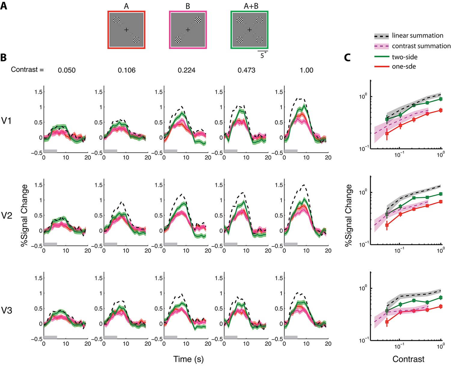
BOLD summation in the absence of neural nonlinearity associated with stimulus summation, with the 6-s stimuli.
(See Figure 3—figure supplement 1 for results obtained with the 1-s stimuli, which are qualitatively identical.) (A) The stimuli used in the BOLD summation experiment. The full stimulus display subtended 24°(w) x 19°(h). Stimulus types A and B are single-sided stimuli, while type A+B is a double-sided stimulus. BOLD responses associated with the outer checkerboard discs were extracted from the corresponding ROIs. These outer discs were of diameter 4° and centered at an eccentricity of 7°. (B) Estimated peristimulus time courses from V1-V3 for the three stimulus types at five different contrast levels. Red and magenta represent responses (lines) and ± SE (bands) to the single-sided stimuli, and green represents responses to the double-sided stimuli. Black dashed lines represent the predictions of linear BOLD summation, which overestimated the measured responses (green bands). Gray bars on the abscissa indicate the duration of the stimulus (6 s). (C) The contrast response functions of V1-V3 as defined by the amplitudes of the time courses. The amplitude of a time course was taken to be the average response between 7–9 s post-stimulus onset when the response typically reached its peak. The red lines represent the average single-sided response amplitudes as a function of luminance contrast. The green lines represent the average double-sided response amplitudes. The gray bands represent the predicted responses (68.2% confidence interval) evoked with the double-sided stimulus under the assumption of linear BOLD summation (i.e. the summed response to conditions A and B), and the magenta bands represent the prediction of contrast summation – the equivalent contrast of a double-sided stimulus being twice that of the corresponding single-sided stimulus. The measured double-sided responses were significantly lower than the predictions of linear BOLD summation and higher than that of contrast summation.
Figure 3—figure supplement 1
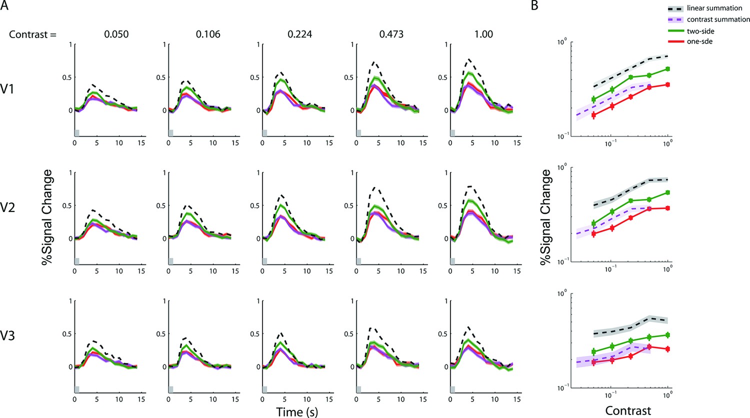
fMRI BOLD summation with a 1-s stimulus duration.
(A) Estimated peri-stimulus BOLD time courses from V1-V3 for the three stimulus types at five contrast levels. Red and magenta curves represent, respectively, the BOLD responses (lines) and ± SE (bands) to the single-sided stimuli, and the green curves represents BOLD responses to the double-sided stimuli. Black dashed lines represent the predictions of linear BOLD summation, which overestimated the measured responses (green bands). Gray bars on the abscissa indicate the duration of the stimulus presentation (1 s). (B) The contrast response functions of V1-V3 as defined by the amplitudes of the time courses. The amplitude of a time course was taken to be the estimated response at 5 s post stimulus onset, when the response typically reached its peak. The red lines represent the averaged response amplitudes to the single-sided stimuli as a function of luminance contrast. Green lines represent the responses to the double-sided stimuli. The dark bands represent the predicted response amplitudes (and 68.2% confidence intervals) evoked with the double-sided stimuli assuming linear BOLD summation, while the magenta bands represent the prediction of contrast summation. Neither of these predictions fits the data. These results are qualitatively identical to those obtained with the 6 s stimulus (Figure 3).
Figure 3—figure supplement 2
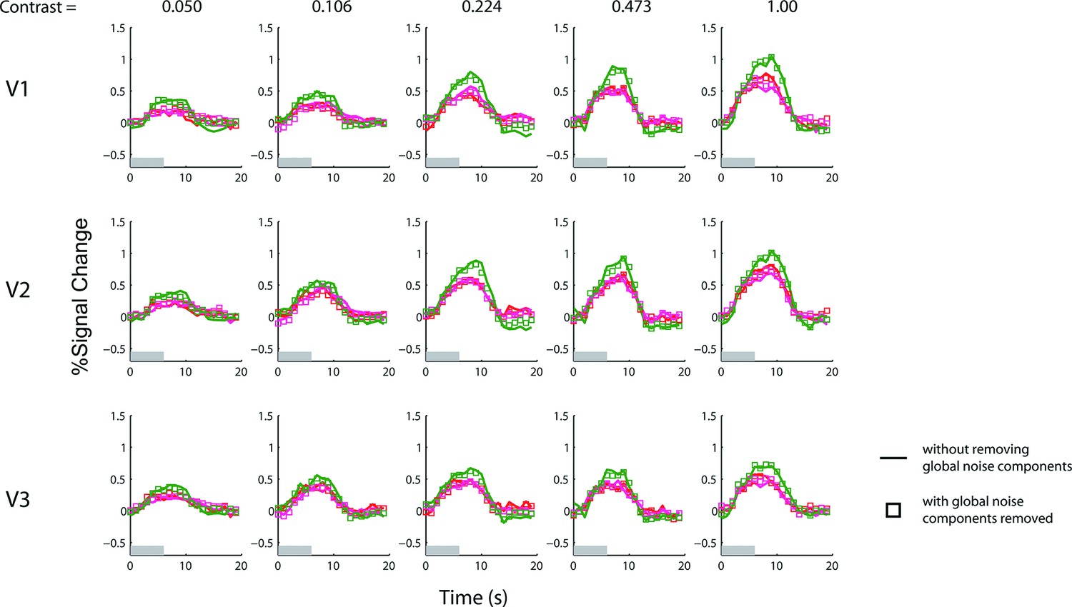
Results of the 6-s BOLD summation experiment with and without removing the global noise components.
The experiment with a 1 s stimulus duration does not have a sufficient signal-to-noise ratio to yield reliable results with conventional deconvolution analysis (using finite-impulse-response basis). The GLM denoising method of Kay et al. (2013) was used to estimate and remove the most prominent principle components of the noise that were shared across voxels. To confirm that this denoising method did not lead to any systematic bias, we applied the same denoising method to the data obtained with the 6 s stimulus duration experiment, for which conventional deconvolution analysis is applicable (Figure 3). The red and magenta colors represent single-sided responses and the green color represents double-sided responses (see also Figure 3). Solid lines, which are identical to those in Figure 3, represent time courses estimated using the conventional deconvolution analysis without adding the estimated global noise components as regressors of no interest (see methods). Square symbols represent the time courses inferred with the global noise components removed by representing them as regressors of no interest. The two methods yielded virtually identical results for the 6-s stimulus.
Figure 3—figure supplement 3
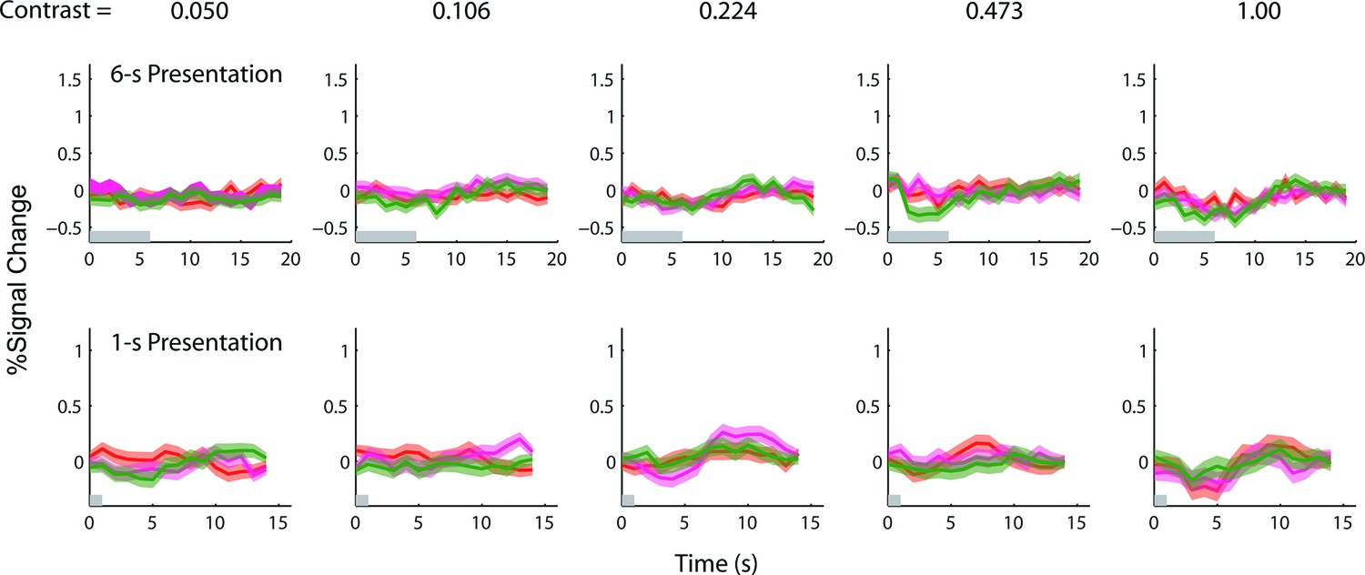
Results of the 1-s and 6-s BOLD summation experiments obtained from the corresponding retinotopically-defined V1 ROI in the left hemisphere of the achiasmic subject.
Red and magenta represent responses (lines) and ± SE (bands) to the single-sided stimuli, and green represents responses to the double-sided stimuli. Since the achiasmic subject viewed the stimuli with only his right eye, there was no stimulus-evoked response in the early visual areas of the left hemisphere. If there were any anticipatory and endogenous response, we should be able to observe the response in the left hemisphere. We found no such response – the peri-stimulus time courses from the left hemisphere do not deviate significantly from zero.
Figure 4 with 2 supplements
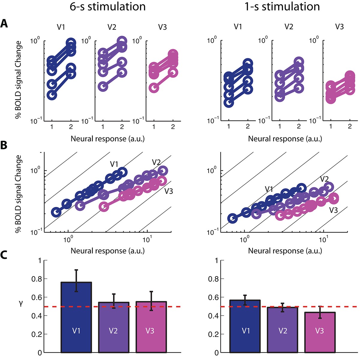
fMRI BOLD signal as a function of neural response.
(A) Five pairs of BOLD response amplitudes evoked in V1-V3 with the single- and double-sided stimulations, each with two stimulus durations, 6-s (left column) and 1-s (right column). If the neural response to a single-sided stimulus is Zi, then the neural response to the corresponding double-sided stimulus will be 2Zi, given our empirical determinations of co-localization and independence of the neuronal populations in an achiasmic visual cortex. (B) The BOLD vs. neural response (BvZ) functions for V1-V3 as inferred by the stitching procedure for the two stimulus durations. The inferred functions can be well fitted with power-law functions (i.e. straight lines in log-log coordinates). These functions are nonlinear, with a log-log slope significantly shallower than unity (the background gray lines). (C) The exponents (γ) of the power-law fit of the BvZ functions for V1-V3. Error bars denote 95% CI. The red line indicates γ = 0.5. γ estimated from V2 and V3 (γ ~ 0.5) were not significantly different, while that obtained from V1 was biased upward, due to a violation of the co-localization assumption (see Discussion) required for inferring the BvZ function using the summation experiment. We thus inferred the (true) BvZ function of V1-V3 using the average γ estimated from V2 and V3 only.
Figure 4—figure supplement 1
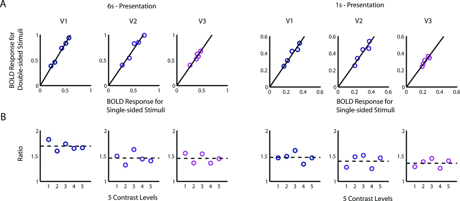
Alternative derivation of the BvZ function.
(A) BOLD amplitudes evoked with a double-sided stimulus were linearly proportional to that evoked with the corresponding single-sided stimulus of the same contrast. There were 5 runs per data point for the 6-s condition and 9 runs for the 1-s condition. For each of the visual areas V1-V3, a linear function provides a good fit the data points [6 s: R2≥0.90; 1 s: R2≥0.85], and the intercepts are not significantly different from zero [nested model comparison for each visual area; 6 s: F(1,3)<0.37, p>0.59; 1 s: F(1,3)<0.27, p>0.64]. (B) Equivalently, contrast had no significant effect on the ratio of BOLD amplitude of a double-sided condition to that of the corresponding single-sided condition [nested model comparison for each visual area, 6 s: F(1,3)<0.53, p>0.52; 1 s: F(1,3)<0.16, p>0.72]. Performing a one-way ANOVA on the BOLD ratios obtained from individual runs also failed to find any significant effect of contrast in any of the visual areas [6 s: F(4,20)<0.37, p>0.8; 1 s: F(4,40)<1.76 p>0.15]. Assuming that the underlying neural responses to the double-sided stimuli is twice those of the corresponding single-sided stimuli, these results imply that the relationship between neural and fMRI BOLD responses follows power law: B = kZγ , where γ can be determined from the ratio of BOLD amplitude evoked by the double-sided stimuli to that evoked by the single-sided ones: γ = log2(B2,i/B1,i). The estimated values of γ from the BOLD ratios are 0.75 (V1), 0.54 (V2), 0.53 (V3) from the 6 s presentation and 0.55 (V1), 0.48 (V2), 0.44 (V3) from the 1 s presentation. These values are very close to those estimated using the stitching procedure (Figure 4C).
Figure 4—figure supplement 2
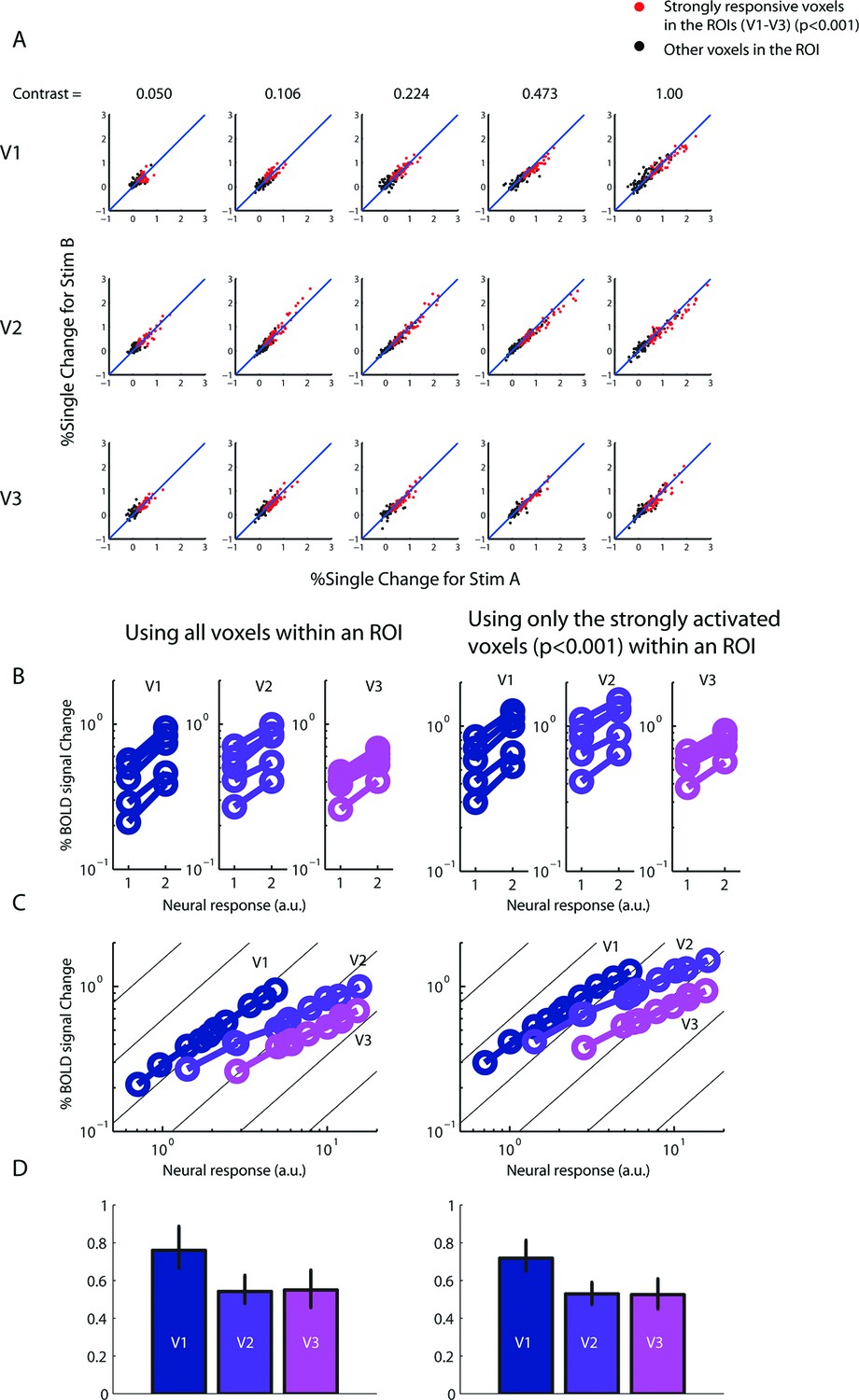
Robustness of BOLD summation results.
(A) BOLD amplitudes of every voxel in each ROI (V1-V3) as evolved by the two versions of the single-sided stimulus (Stim A and B of Figure 3) in the 6-s experiment. The voxels responded approximately equally to both versions of the stimulus, indicating that any imperfect homotopy and/or gaze control did not significantly affect the stimuli's ability to equally co-activate the voxels. Red dots represent voxels in the ROIs that were strongly responsive (uncorrected p<0.001) to both versions of the stimulus. Reanalyzing the data using only these strongly responsive voxels yielded essentially the same results as in Figure 4 when all the voxels with the ROIs were used (right vs. left column, respectively, of B–D.
Figure 5

Comparisons between neural response inferred from the BvZ function (B = kZγ) and single-unit spiking activity.
(A) Neural contrast response functions. The black dots and line are the average single-unit firing rate as a function of luminance contrast recorded in macaque V1 (replotted from Albrecht, 1995) and the best fitting Naka-Rushton function (Naka and Rushton, 1966), respectively. Red open and filled circles represent the BvZ-inferred neural contrast responses in V1 of the achiasmic subject, computed from our 6-s and 1-s single-sided BOLD data sets (from Figure 3 and Figure 3—figure supplement 1) and matched to single-unit firing rates with a single scaling constant to align the data point at contrast = 1. Gray open and filled triangles represent the linearly scaled BOLD contrast responses from the same data sets. The BvZ-inferred neural responses are in excellent agreement with the single-unit spiking data, whereas linearly scaled BOLD responses are not. (B) fMRI BOLD contrast responses from 21 published data sets (a-u; see Table 1) were individually matched to the single-unit spiking responses function of (A), assuming a power-law function to convert BOLD response to spike rate. The fits were good, with R2 ranging from 0.73 to 0.99. The distribution of the best-fitting exponents (γ) is shown in (C). The median of the distribution (0.48) is close to the exponent (0.5, red dashed vertical line) of the BvZ function inferred from the achiasmic subject. Asterisk (*) marks studies in which subjects attended to the stimuli used to obtain the contrast response functions. Underline (_) marks studies that measured and analytically discounted any task-related baseline response from the contrast response functions. (D,E) An otherwise identical analysis as in (B,C) but using the single-unit (spike rate) contrast response function obtained from Heeger et al. (2000) instead of the single-unit contrast responses function used in (A) from Abrecht (1995). (Note that some data points are out of the ordinate range in B and D; they are omitted from the plots.)
Tables
Table 1
Data sources of Figure 5.
| Legend | Publication | Figure # (Condition) | Subjects | γ (Figure 5B ) | γ (Figure 5D ) | R2 (Figure 5B ) | R2 (Figure 5D ) |
|---|---|---|---|---|---|---|---|
| a | Pestilli et al., 2011 | Figure 4B (Focal Cue – non Target) | Human | 0.50 | 0.64 | 0.77 | 0.86 |
| b* | Pestilli et al., 2011 | Figure 4B (Focal Cue - Target) | Human | 0.15 | 0.21 | 0.93 | 0.94 |
| c* | Pestilli et al., 2011 | Figure 4B (Distributed Cue –Target) | Human | 0.24 | 0.34 | 0.79 | 0.88 |
| d* | Pestilli et al., 2011 | Figure 4B (Distributed Cue – non Target) | Human | 0.25 | 0.37 | 0.85 | 0.93 |
| e* | Avidan et al., 2002 | Figure 2B (Faces) | Human | 0.61 | 0.72 | 0.96 | 0.93 |
| f* | Avidan et al., 2002 | Figure 2B (Objects) | Human | 1.06 | 1.24 | 0.91 | 0.89 |
| g* | Buracas & Boynton 2007 | Figure 1 | Human | 0.32 | 0.40 | 0.93 | 0.98 |
| h* | Boynton et al., 1999 | Figure 3 and Figure 4 | Human | 0.64 | 0.84 | 0.97 | 0.99 |
| i | Schumacher et al., 2011 | Figure 4A (gradient echo) | Human | 0.28 | 0.38 | 0.73 | 0.85 |
| j | Schumacher et al., 2011 | Figure 4A (spin echo) | Human | 0.28 | 0.36 | 0.86 | 0.93 |
| k | Schumacher et al., 2011 | Figure 4C (gradient echo) | Human | 0.56 | 0.66 | 0.97 | 0.98 |
| l | Schumacher et al., 2011 | Figure 4C (spin echo) | Human | 0.40 | 0.50 | 0.91 | 0.96 |
| m | Li et al., 2008 | Figure 3 (Unattended) | Human | 0.65 | 0.75 | 0.99 | 0.96 |
| n* | Li et al., 2008 | Figure 3 (Attended) | Human | 0.26 | 0.36 | 0.91 | 0.85 |
| o | Moradi & Heeger 2009 | Figure 2 | Human | 0.25 | 0.37 | 0.86 | 0.83 |
| p* | Olman et al., 2004 | Figure 4A (Natural Images) | Human | 0.34 | 0.50 | 0.97 | 0.97 |
| q* | Olman et al., 2004 | Figure 4A (Whitened Images) | Human | 0.48 | 0.68 | 0.99 | 0.97 |
| r | Park et al., 2008 | Figure 9 | Human | 0.61 | 0.70 | 0.98 | 0.94 |
| s | Tootell et al., 1998 | Figure 5 | Human | 0.71 | 0.87 | 0.89 | 0.94 |
| t* | Zenger-Landolt & Heeger 2003 | Figure 9 (Without Surround) | Human | 0.75 | 0.83 | 0.85 | 0.93 |
| u | Logothetis et al., 2001 | Figure 5B (BOLD) | Monkey | 0.65 | 0.68 | 0.75 | 0.88 |
-
Asterisk (*) marks indicate studies in which subjects attended to the stimuli used to obtain the contrast response functions.
-
Underline (_) marks indicate studies that measured and analytically discounted any task-related baseline response from the contrast response functions.
Download links
A two-part list of links to download the article, or parts of the article, in various formats.
Downloads (link to download the article as PDF)
Open citations (links to open the citations from this article in various online reference manager services)
Cite this article (links to download the citations from this article in formats compatible with various reference manager tools)
Using an achiasmic human visual system to quantify the relationship between the fMRI BOLD signal and neural response
eLife 4:e09600.
https://doi.org/10.7554/eLife.09600


