Internal models for interpreting neural population activity during sensorimotor control
- Carnegie Mellon University, United States
Figures
Figure 1 with 1 supplement

Closed-loop control of a brain-machine interface (BMI) cursor.
(A) Schematic view of the brain-machine interface. Subjects produce neural commands to drive a cursor to hit visual targets under visual feedback. (B) Cursor trajectories from the first 10 successful trials to each of 16 instructed targets (filled circles) in representative data sets. Target acquisition was initiated when the cursor visibly overlapped the target, or equivalently when the cursor center entered the cursor-target acceptance zone (dashed circles). Trajectories shown begin at the workspace center and proceed until target acquisition. Data are not shown during target holds.
Figure 1—figure supplement 1
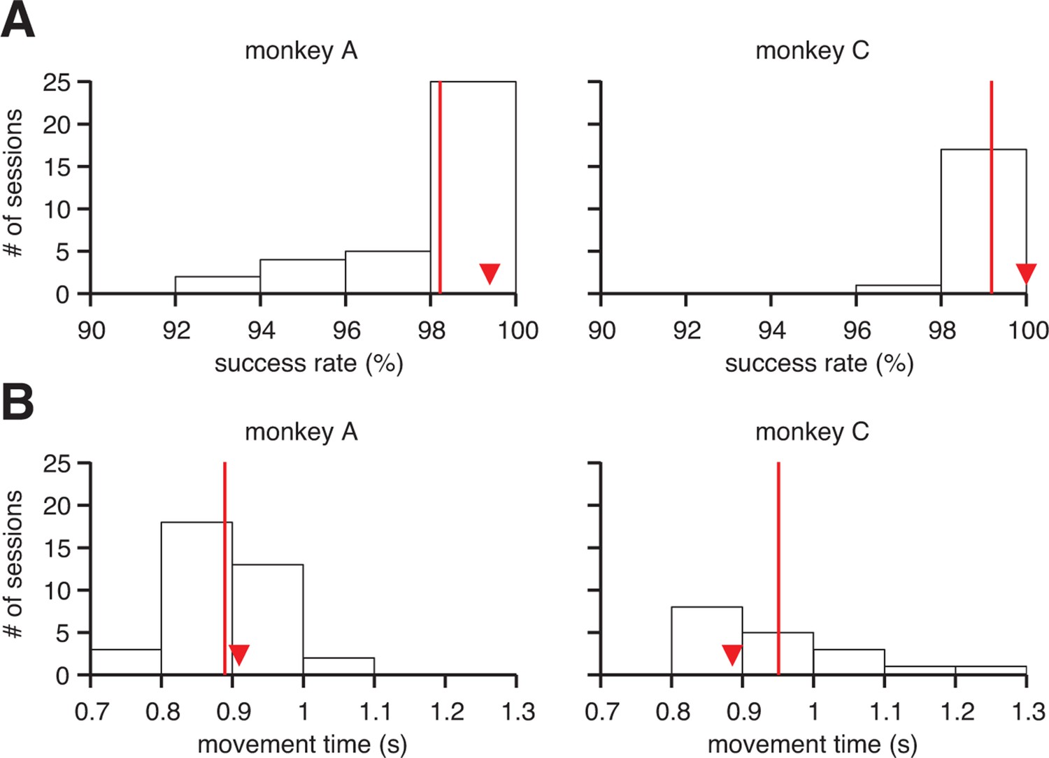
Proficient control of the brain-machine interface (BMI).
(A) Histograms of within-session averaged success rates and (B) movement times across all sessions and both monkeys. Red lines denote averages across sessions, and triangles indicate the within-session averages for the example sessions from Figure 1B. Movement times were calculated as the time elapsed between target onset and target acquisition (i.e., excluding all hold times, but including reaction times).
Figure 2 with 1 supplement

Subjects compensate for sensory feedback delays while controlling a BMI.
(A) The visuomotor latency experienced by a subject in our BMI system was assessed by measuring the elapsed time between target onset and the first significant () decrease in angular error. If that first decrease was detected timesteps following target onset, we concluded that the visuomotor latency was at least timesteps (red dashed lines). For both subjects, the first significant difference was highly significant (**, two-sided Wilcoxon test with Holm-Bonferroni correction for multiple comparisons; = 5908 trials; monkey C: = 4578 trials). (B) Conceptual illustration of a single motor command (black arrows) shifted to originate from positions lagged relative to the current cursor position (open circle). In this example, the command points farther from the target as it is shifted to originate from earlier cursor positions. (C) Motor commands pointed closer to the target when originating from the current cursor position (zero lag) than from outdated (positive lag) cursor positions that could be known from visual feedback alone (**, two-sided Wilcoxon test; monkey A: = 33,660 timesteps across 4489 trials; monkey C: = 31,214 timesteps across 3639 trials). Red lines indicate subjects’ inherent visual feedback delays from panel A. Shaded regions in panels A and C (barely visible) indicate SEM.
Figure 2—figure supplement 1
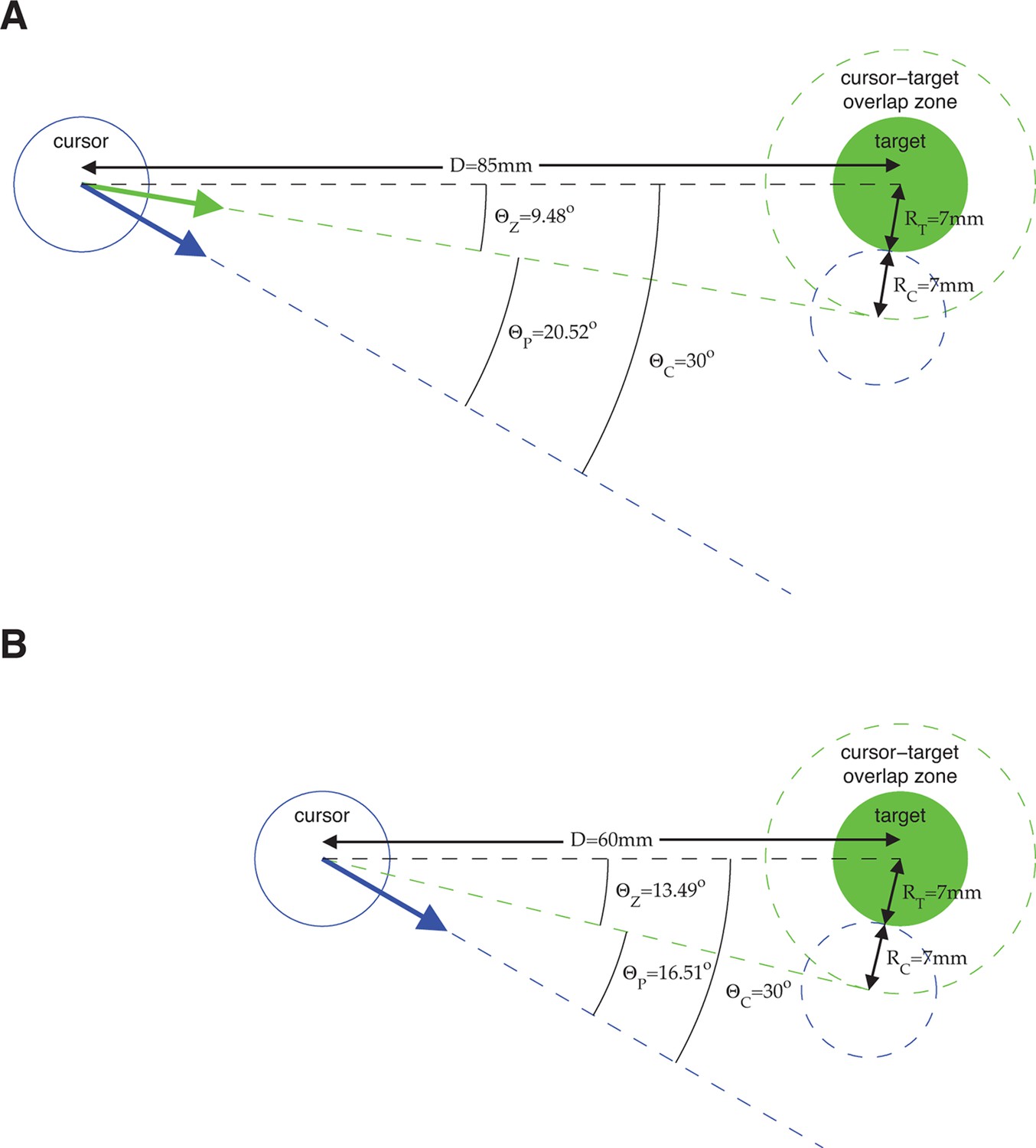
Error metrics for assessing estimates of movement intent.
The primary error metric we used was the absolute angle by which a velocity command would have missed the target, taking into account the cursor and target radii. Because task success requires hitting the target (i.e., cursor-target overlap), we define all commands that would result in cursor-target overlap as having zero angular error. Mathematically, this corresponds to any velocity command that points within degrees from the target center, where is the distance between target center and the position from which the velocity command originates, and and are the cursor and target radii, respectively. A velocity command that would not hit the target is given an error, , equal to the angle by which the cursor would have missed the target. Equivalently, we can consider the cursor-target overlap zone defined by a target-concentric circle with radius , and define angular error, , to be the smallest angle between the velocity command and the perimeter of the cursor-target overlap zone. (A) Consider an example in which we assess the error of velocity commands (blue and green arrows) originating from a position mm from the target center (the distance between workspace center and target center in a typical experiment). Here, the cursor radius, , and the target radius, , are both 7 mm (typical values from experiments). Any velocity command that points within of the target center would result in cursor-target overlap and thus would be evaluated as having zero angular error. The green arrow points in the direction farthest from the target center such that movement of the cursor (dashed blue circle) in this direction would result in cursor-target overlap. A velocity command (blue arrow) pointing from the target center would miss the cursor-target overlap zone by . (B) Consider a similar example, but with the velocity command originating from a position mm from the target center. Because the cursor-target distance has decreased, the zero error window increases to . As a result, a velocity command that points from the target center (blue arrow; same as in panel A), is now evaluated as having a smaller error, . The difference between the error angles, , in panel A and panel B, reflects the task goals, because a wider range of velocity commands would result in task success in panel B compared to panel A, and thus the same velocity command is more task-appropriate in panel B than in panel A. The metric was used extensively throughout this work (Figure 2A,C, Figure 3B,C, Figure 4C, Figure 6A, Figure 3—figure supplement 3, Figure 3—figure supplement 4, Figure 3—figure supplement 7, Figure 3—figure supplement 8, and Figure 4—figure supplement 2). We repeated those analyses using as the error metric (i.e., ignoring the distance to the target, cursor radius, and target radius) and found qualitatively similar results. In Figure 2C and Figure 3—figure supplement 8, velocity commands were evaluated as originating from a range of lagged cursor positions. Since cursor positions later in a trial tend to be closer to the target than earlier positions, velocity commands will tend to have smaller when originating from these later cursor positions. We controlled for this distance-to-target effect to ensure that it did not influence our results (see Materials and methods).
Figure 3 with 8 supplements
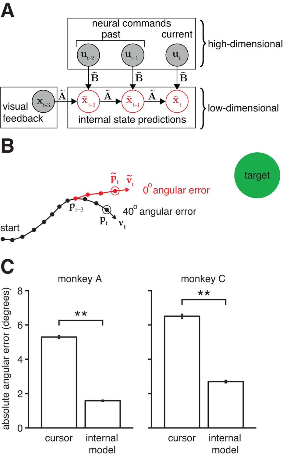
Mismatch between the internal model and the BMI mapping explains the majority of the subjects’ cursor movement errors.
(A) At each timestep, the subject’s internal state predictions () are formed by integrating the visual feedback () with the recently issued neural commands () using the internal model (). We defined cursor states and internal state predictions to include components for position and velocity (i.e., ). (B) Cursor trajectory (black line) from a BMI trial that was not used in model fitting. Red whisker shows the subject’s internal predictions of cursor state as extracted by IME. The critical comparison is between the actual cursor velocity (; black arrow) and the subject’s internal prediction of cursor velocity (; red arrow). (C) Cross-validated angular aiming errors based on IME-extracted internal models are significantly smaller than cursor errors from the BMI mapping (**, two-sided Wilcoxon test; monkey A: = 5908 trials; monkey C: = 4577 trials). Errors in panel B are from a single timestep within a single trial. Errors in panel C are averaged across timesteps and trials. Errors in panels B and C incorporate temporal smoothing through the definition of the BMI mapping and the internal model, and are thus not directly comparable to the errors shown in Figure 2C, which are based on single-timestep velocity commands needed for additional temporal resolution. Error bars (barely visible) indicate SEM.
Figure 3—figure supplement 1
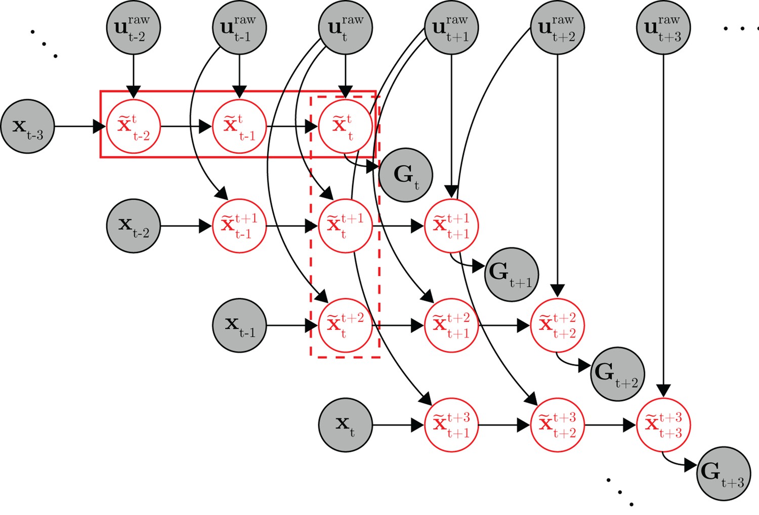
Full probabilistic graphical model for the internal model estimation (IME) framework.
At timestep , the subject generates a set of internal state predictions (row of variables in the solid box) based on the most recently available visual feedback () and recently issued neural commands (). Because the subject aims straight to the target from the subject’s up-to-date prediction of cursor position, the target position () should lie along the line defined by subject’s up-to-date position and velocity predictions ( and , included in ). At the next timestep (), the subject generates a revised set of internal predictions (row of variables) based on newly received visual feedback (), the most recently issued neural command (), and previously issued neural commands ( and ). A column of internal state predictions represents the subject’s internal predictions given more and more recent visual feedback (e.g., the variables in the dashed box represent the subject’s internal predictions of the timestep cursor state given visual feedback available through timestep ). Once a neural command is issued, it cannot be revised, and as such, the same neural command continues to influence internal predictions until visual feedback becomes available from the corresponding timestep ( affects the , and variables, but not the variables as has become available, rendering irrelevant). The target position took on the same value for all timesteps within the same trial. Shaded nodes indicate observed data, and red unshaded nodes are latent variables representing the subject’s internal state predictions.
Figure 3—figure supplement 2
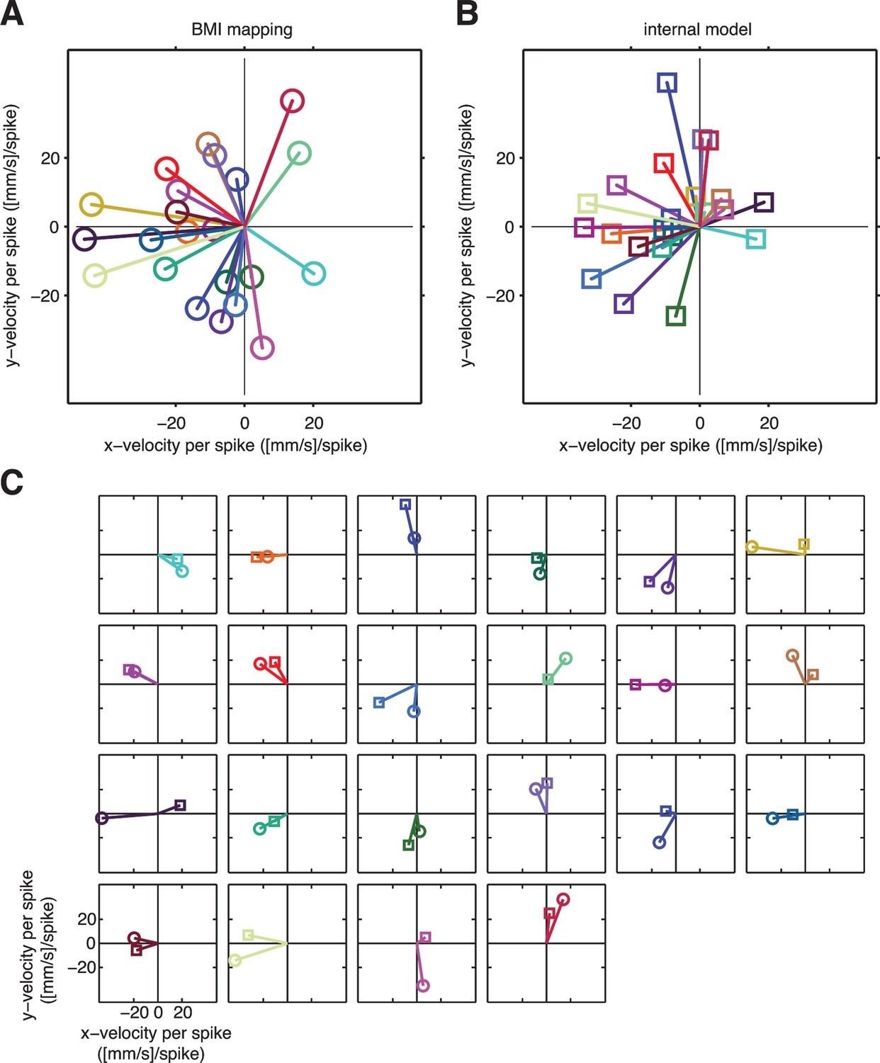
A unit-by-unit comparison of the subject’s internal model and the BMI mapping.
Both the internal model and the BMI mapping can be visualized as a collection of pushing vectors. (A) The BMI mapping parameter from Equation 1 describes how each neuronal unit actually drove the BMI cursor. Each 2D column in the velocity portion (lower two rows) of corresponds to a particular unit and can be visualized as a pushing vector describing the direction and magnitude by which a single spike from that unit would push the cursor according to the BMI mapping. Each unit’s pushing vector is given a unique color. (B) The internal model parameter from Equation 2 describes how the subject believes each neuronal unit drives the cursor. As in panel A, each 2D column of the velocity portion of corresponds to a particular unit. Pushing vectors corresponding to the same unit in panel A and panel B are given the same color. See Visualizing an extracted internal model for additional details on the pushing vectors in panels A and B. (C) Unit-by-unit comparison of pushing vectors from the BMI mapping (circles) and internal model (squares) from panel A. When looking across all units, there was no consistent structure in the differences between pushing vectors through the internal model versus through the BMI mapping. Some units’ pushing vectors were similar through the BMI mapping and the subject’s internal model, whereas other units’ pushing vectors showed substantial differences. Despite these differences, some patterns of neural activity resulted in similar velocities through the internal model and the BMI mapping (Figure 4A), whereas other patterns resulted in different velocities (Figure 4B). Analyzing the high-dimensional population activity enabled the identification of these effects, which could not have been revealed by analyzing the low-dimensional behavior or individual units in isolation. Parameters visualized in panels A–C were taken from representative session A010609.
Figure 3—figure supplement 3
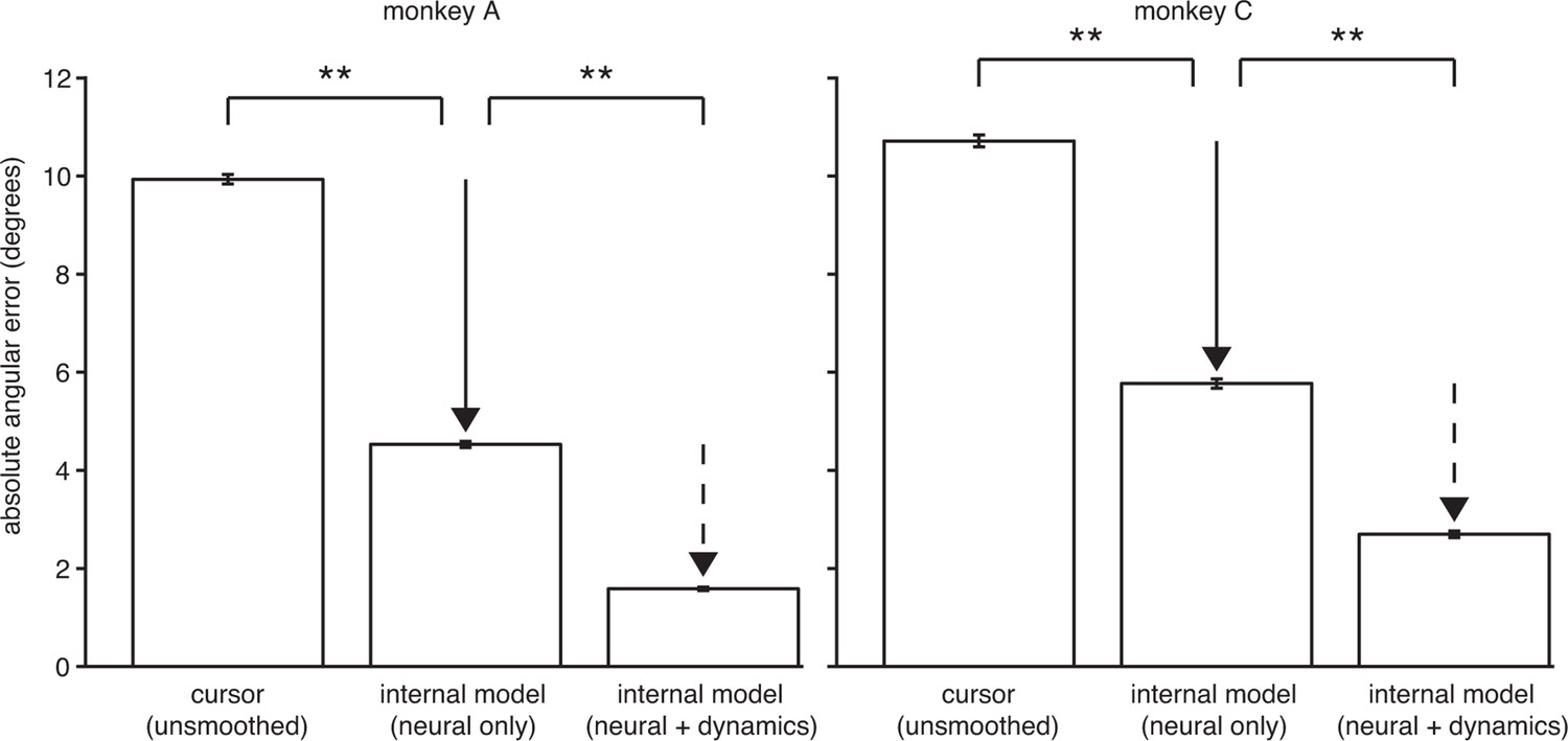
The explanatory power of IME comes primarily from structure in the high-dimensional neural activity.
IME explains cursor errors by identifying two main types of statistical structure in the data. The two types of structure are (i) temporal structure in the dynamics of low-dimensional velocities (), and (ii) hidden, task-appropriate structure in the high-dimensional neural activity (). Here we asked to what extent each type of structure contributes toward IME’s overall explanatory power. In the internal model of Equation 10, summarizes temporal dynamics in the low-dimensional velocity predictions, including how velocity feedback informs internal predictions of cursor state and the degree of temporal smoothness across internal velocity predictions within a single whisker. Intended velocity tends to be similar from one timestep to the next, and whiskers with the appropriate temporal structure (as determined by fitting to the data) can explain a portion of cursor movement errors. The internal model parameters and reveal features in the high-dimensional neural activity that are consistent with straight-to-target movement intent and that are often not reflected in the BMI cursor movements. To determine the relative contribution of structure in the high-dimensional neural data toward the explanatory power of IME, we devised a constrained variant of IME that relies entirely on the high-dimensional neural activity to generate whiskers. Specifically, we constrained in Equation 6, removing IME’s ability to leverage velocity dynamics within its whiskers while preserving its ability to identify structure in the high-dimensional neural activity (since no constraints are placed on ). In this constrained IME variant, termed “neural-only” IME, the subject’s internal prediction of the velocity resulting from neural command is simply . Because neural-only IME does not incorporate temporal smoothing of velocity predictions, it cannot be directly compared to the BMI mapping via the cursor error presented in Figure 3C, which was computed using smoothed cursor velocities. To enable fair comparison with the BMI mapping, we computed cursor errors using single-timestep (unsmoothed) velocity commands, (replicated from Equation 8). Here we compared the angular errors of these (“neural only”) and (“unsmoothed cursor”). Internal models extracted using neural-only IME explain 54% and 46% of unsmoothed cursor errors in monkeys A and C, respectively, demonstrating that there is considerable structure in the high-dimensional neural activity. For reference, we also include the error from unconstrained IME (i.e., by fitting to the data; “neural + dynamics”; replicated from Figure 3C). In this view, the large difference between unsmoothed cursor errors and neural-only internal model errors (solid arrow) represents the explanatory power of the structured high-dimensional neural activity without applying any temporal smoothing and without leveraging visual feedback of cursor velocity. The smaller difference between errors through the neural-only internal model and the unconstrained internal model (dashed arrow) demonstrates the additional explanatory power gained by incorporating velocity feedback and temporal smoothing. As in Figure 3C, angular error was defined as the angle by which the cursor would have missed the cursor-target overlap zone had it continued in the direction of (BMI mapping) or (internal model) from position or , respectively (i.e., in Figure 2—figure supplement 1). Absolute angular errors were first averaged within each trial, then averaged across all trials. Error bars indicate SEM (**: , two-sided Wilcoxon test; monkey A: = 5908 trials; monkey C: = 4577 trials).
Figure 3—figure supplement 4
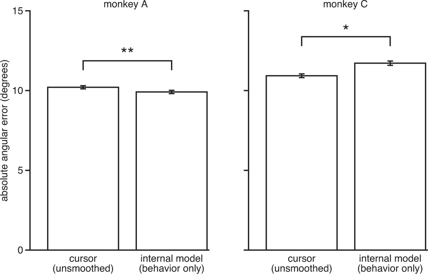
IME does not explain cursor errors when fit to low-dimensional behavior.
We fit neural-only IME using low-dimensional behavior (i.e., cursor velocity) in place of the high-dimensional neural activity. Extracted internal models result in errors similar to or even larger than those of the BMI cursor (i.e., internal model errors are not substantially smaller than cursor errors, as in Figure 3C). This suggests that the explanatory power of the IME framework is largely due to reliable structure in the high-dimensional neural activity, as opposed to structured errors in the low-dimensional behavior. Further, these results suggest that our ability to identify internal model mismatch might not have been possible given only behavioral measurements. Error bars indicate SEM (*: ; **: , two-sided Wilcoxon test; monkey A: = 5908 trials; monkey C: = 4577 trials).
Figure 3—figure supplement 5
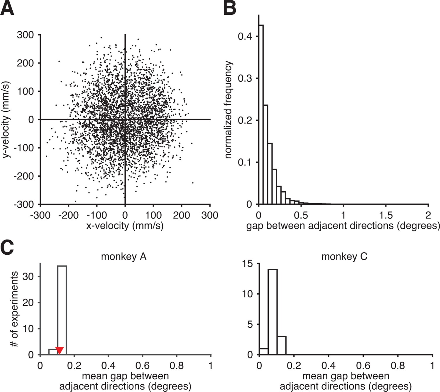
Subjects could readily produce the entire range of movement directions through the BMI mapping.
(A) Observed movement velocities from representative session A072208. Velocities were computed using single-timestep spike counts (i.e., from Equation 8). (B) The distribution of gaps between adjacent observed movement directions from panel A. (C) The distribution of the mean within-session direction gap across all intuitive sessions. Red triangle indicates the mean gap from the data in panel B. Since movement direction can be noisy at low speeds, we also analyzed these distributions after withholding observed velocities with low speed (i.e., points near the origin in panel A). Results (as in panels B and C) were nearly identical (data not shown).
Figure 3—figure supplement 6
Internal model mismatch is not an artifact of correlated spiking variability.
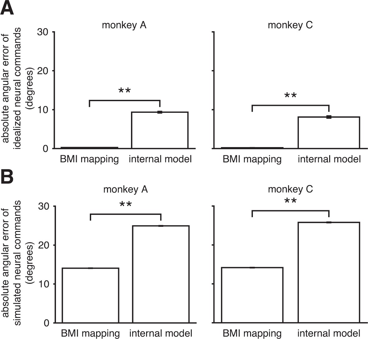
To determine whether our finding of internal model mismatch could be an artifact of correlated spiking variability, we simulated noisy neural commands according to the alternate hypothesis that the internal model was well-matched to the BMI mapping. We could then ask whether our main finding of internal model mismatch (Figure 3C) could be explained by the properties of the noise in the real data. Under this alternative hypothesis, the subject generates idealized neural commands that, prior to corruption by noise, would produce the desired movement direction through the BMI mapping. We simulated these idealized neural commands and their noisy counterparts by sampling from the recorded neural activity (see Assessing whether internal model mismatch could appear as a spurious result due to correlated spiking variability). (A) By construction, the idealized neural commands had near-zero errors through the BMI mapping. When interpreted through the extracted internal model, those patterns produced substantially larger errors. (B) After corruption by noise, which was matched to the statistics of the recorded neural activity, simulated neural commands had substantially larger errors through the extracted internal model than through the BMI mapping. Thus when assuming the alternative hypothesis, simulation results contrast with the results from the real data (Figure 3C). Furthermore, errors increased by roughly the same amount through both the BMI mapping and the internal model. Taken together, these simulation results suggest that our main finding of internal model mismatch cannot simply be explained by extracted internal models that were better fit to the noise properties of the real data, relative to the BMI mapping. Error bars (barely visible) indicate SEM (**, two-sided Wilcoxon test; panel A: = 1152 (monkey A) and = 576 (monkey C) idealized neural commands; panel B: = 125,459 (monkey A) and = 102,689 (monkey C) simulated neural commands).
Figure 3—figure supplement 7
IME does not explain cursor errors when fit to neural commands that do not contain high-dimensional structure.
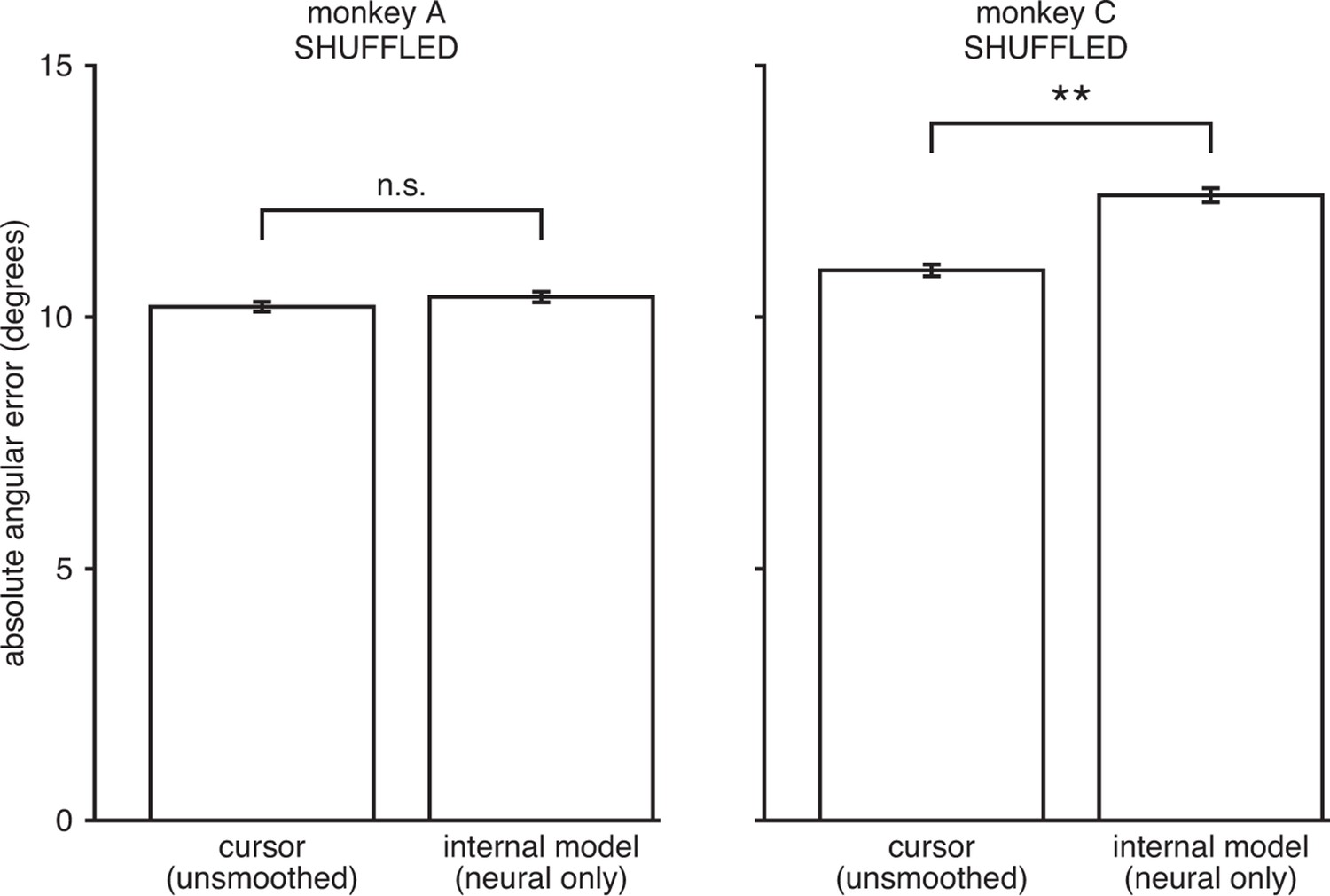
We applied neural-only IME to datasets in which we shuffled the neural activity in the null-space of , while preserving the neural activity in the row-space of . By design, these shuffled datasets result in exactly the same velocities through the BMI mapping (“unsmoothed cursor” bars here exactly match those in Figure 3—figure supplement 3). However, any remaining structure in the high-dimensional neural activity is scrambled and as such cannot be leveraged by IME to explain errors. As shown, internal models extracted by neural-only IME from the shuffled data result in errors similar to or even larger than those from the BMI cursor. These results further demonstrate that the explanatory power of the IME framework is largely due to reliable structure in the high-dimensional neural activity and not due to overfitting noise in the data. Error bars indicate SEM (n.s.: not significant, ; **, two-sided Wilcoxon test; monkey A: = 5908 trials; monkey C: = 4577 trials).
Figure 3—figure supplement 8
A simplified alternative internal model is not consistent with the data.
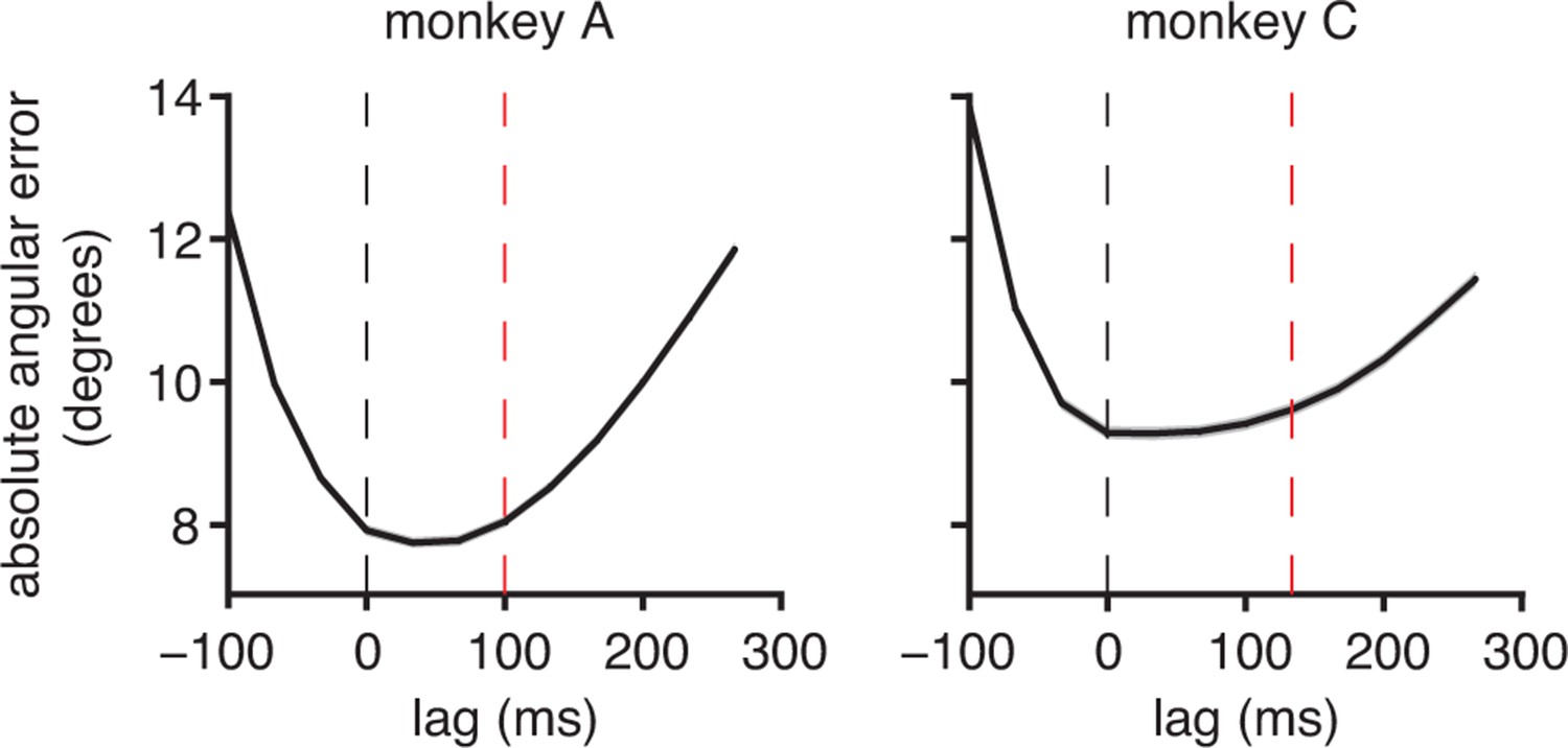
The central principles of the IME framework are that the subject internally predicts the current cursor position based on an internal model, and the subject aims straight to the target from that predicted position through the internal model. We asked whether we could account for the data using a simpler form of the internal model, which incorporates straight-to-target aiming without internal prediction. In this alternative model, the subject aims straight to the target from the most recent cursor position available from visual feedback, rather than from an internal forward prediction of cursor position. As in IME, this “aim-from-feedback” approach involves an internal model that need not match the BMI mapping. We fit this model via linear regression using the same feedback delays determined from the BMI behavior ( from Figure 2A). At timestep , the intended aiming direction was assumed to be straight to the target center from the feedback cursor position, , and intended speed was taken to match that of the single-timestep velocity command through the BMI mapping, . These aiming directions were regressed against single-timestep spike counts, i.e., the corresponding , to yield an internal model. Internal models were fit and errors were evaluated using the same cross-validation practices used to evaluate the IME framework. Shaded regions (barely visible) indicate SEM (monkey A: = 33,660 timesteps across 4489 trials; monkey C: = 31,214 timesteps across 3639 trials). If subjects intend to drive the cursor from the position given by the most recent visual feedback, internal models fit according to this aim-from-feedback principle should predict intended velocities that point closest to targets when originating from feedback cursor positions (i.e., cursor positions that lag the recorded neural activity by timesteps). This was not the case. We found that internal models fit according to the aim-from-feedback principle result in cross-validated velocity commands that point closest to targets when originating from cursor positions more recent than those from the most recently available visual feedback (i.e., curves do not have clear minima at the red lines). This finding is consistent with subjects aiming straight to the target from an up-to-date internal prediction of the current cursor position (Figure 2C). Because of mismatch between the subject’s internal model and the BMI mapping, the subject’s up-to-date estimate of cursor position need not match the actual current cursor position, and as such, we should not necessarily expect minima in these curves at lag = 0. Given this evidence that subjects perform some sort of internal tracking, we implemented a number of different internal models to dissect the exact form of that tracking process. Specifically, we implemented internal models that perform no tracking (aim-from-feedback, presented here), tracking without previously issued motor commands (data not shown), and tracking with previously issued motor commands (main results, which use Equations 9–13), among others. Empirically, these internal models all yield similar cross-validated errors. The explanation for this similarity is that the different formulations identify similar high-to-low dimensional mappings that capture the subject’s intent to move straight to the target, and the direction of these intended commands tends to dominate any effect of the position from which those commands originate. This reasoning is consistent with our finding that cursor errors are better explained by structure in the high-dimensional neural activity than by temporal structure in the cursor kinematics (Figure 3—figure supplement 3), structure in low-dimensional behavior (Figure 3—figure supplement 4), or low-dimensional structure in the recorded neural activity (Figure 3—figure supplement 7). We ultimately chose to present results from the internal model of Equations 9–13 because it performs as well as any internal model we tested, and its formulation is consistent with a number of prominent studies evidencing the use of internal copies of motor commands (Sommer, 2002; Scott, 2004; Miall et al., 2007; Crapse and Sommer, 2008; Shadmehr and Krakauer, 2008; Sommer and Wurtz, 2008; Huang et al., 2013; Azim et al., 2014).
Figure 4 with 2 supplements
Neural activity appears correct through the internal model, regardless of how the actual cursor moved.
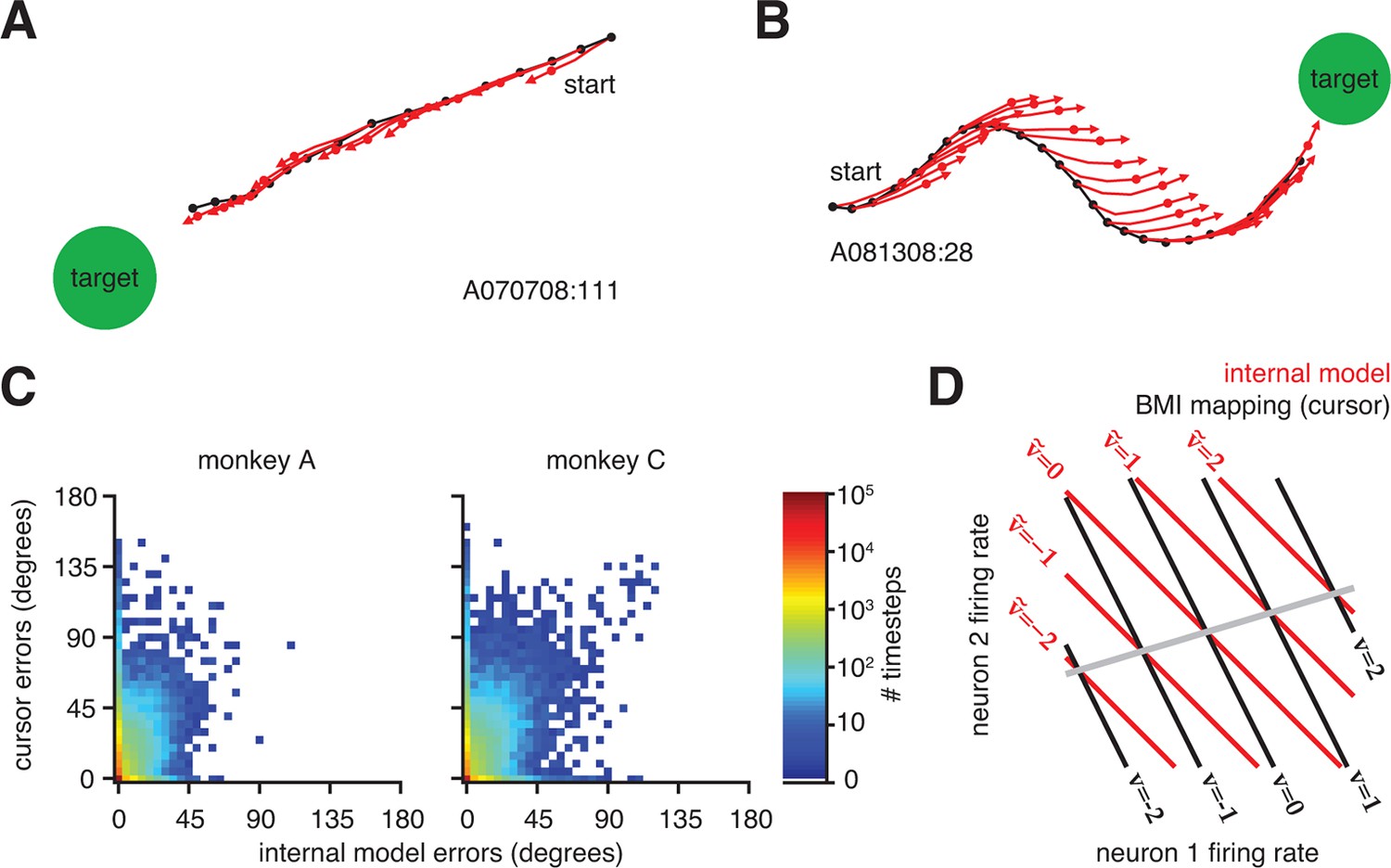
(A) Typical trial in which the cursor followed a direct path (black) to the target. Internal model predictions (red whiskers) also point straight to the target. (B) Trial with a circuitous cursor trajectory. Internal model predictions point straight to the target throughout the trial, regardless of the cursor movement direction (same color conventions as in panel A). (C) Timestep-by-timestep distribution of BMI cursor and internal model errors. Neural activity at most timesteps produced near-zero error through the internal model, despite having a range of errors through the BMI mapping. (D) Hypothetical internal model (red) and BMI mapping (black) relating 2D neural activity to a 1D velocity output. This is a simplified visualization of Equations 1 and 2, involving only the and parameters, respectively. Each contour represents activity patterns producing the same velocity through the internal model (, red) or BMI mapping (, black). Because of internal model mismatch, many patterns result in different outputs through the internal model and the BMI. However, some patterns result in the same output through both the internal model and the BMI (gray line). Here we illustrate using a 2D neural space and 1D velocity space. In experiments with -dimensional neural activity and 2D velocity, activity patterns producing identical velocities through both the internal model and the cursor span a -dimensional space.
Figure 4—figure supplement 1
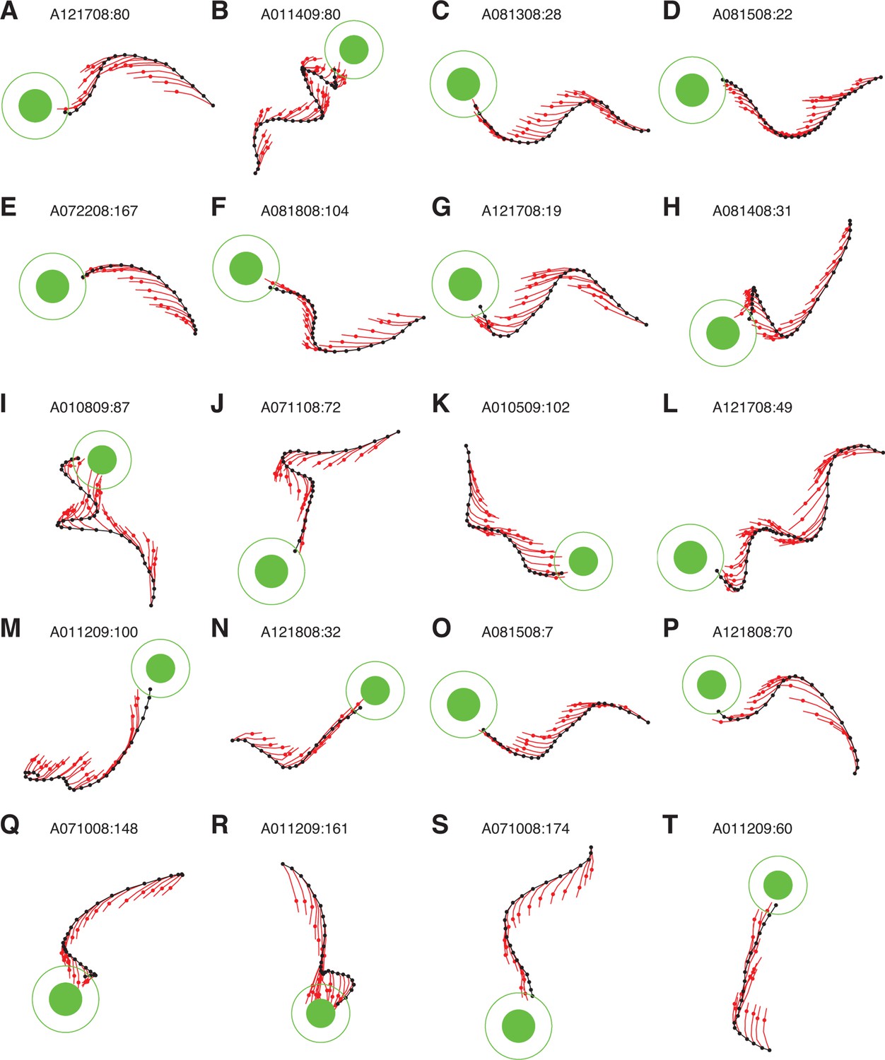
IME whiskers consistently point to the target regardless of cursor movement direction.
Additional example cursor trajectories (black) are overlaid with cross-validated predictions from extracted internal models (red whiskers), as in Figure 4A,B. Each trial was held-out when fitting the internal model used to generate its whiskers. Each whisker shows the subject’s internal belief of how the cursor trajectory evolved, beginning from the most recently available visual feedback of cursor position (black dots) to the subject’s up-to-date prediction of the current cursor position (red dots). The final whisker segments (red line beyond each red dot) represent the subject’s intended velocity command. Trials were selected to highlight differences between extracted internal models and the BMI mappings. In these trials, black cursor trajectories at times appear irrational with respect to targets, yet internal models reveal whiskers that consistently point toward the targets. Averaged cursor and internal model errors within each of these trials are shown in Figure 4—figure supplement 2.
Figure 4—figure supplement 2
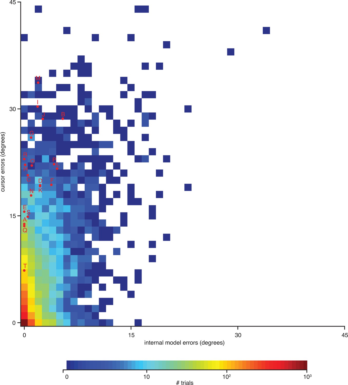
Errors from trials in Figure 4—figure supplement 1 highlighted on the distribution of errors across trials.
Letters correspond to trials from Figure 4—figure supplement 1. Format is similar to that of Figure 4C, but there histograms were constructed from single-timestep errors. Here, errors were averaged across all timesteps within each trial, allowing for direct correspondence to the trials shown in Figure 4—figure supplement 1. Data are from monkey A only. Monkey C data are qualitatively similar (data not shown).
Figure 5 with 1 supplement

Internal model mismatch limits the dynamic range of BMI cursor speeds.
(A) BMI cursor speeds across the range of intended (i.e., internal model) speeds. At low intended speeds, BMI speeds were higher than intended, whereas for mid-to-high intended speeds, BMI speeds were lower than intended. Shaded regions indicate SEM. (B) During the hold period prior to target onset, intended speeds were significantly lower than those produced through the BMI mapping. During movement, intended speeds were significantly higher than those produced through the BMI. Error bars indicate SEM (**, two-sided Wilcoxon test; monkey A: trials; monkey C: trials). In panels A and B internal models were used to predict intended speed on trials not used during model fitting.
Figure 5—figure supplement 1
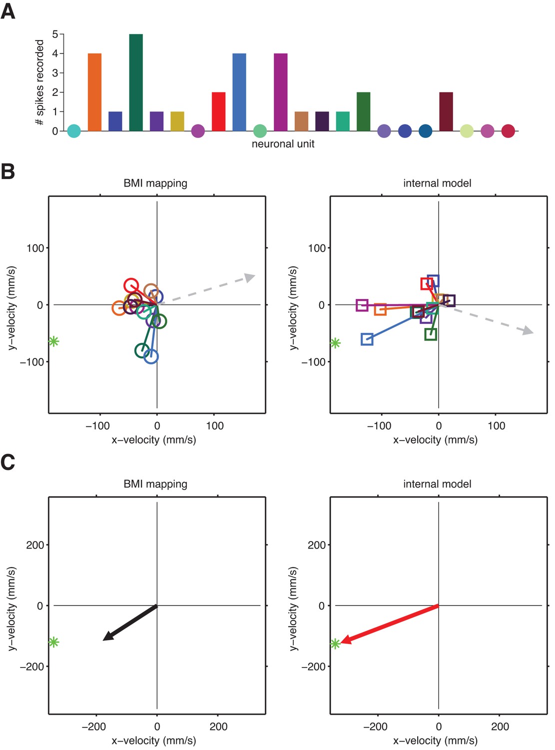
A unit-by-unit example of internal model mismatch limiting cursor speed dynamic range.
(A) Spike counts during a single example timestep across 22 units. Circles indicate a zero spike count. This example timestep was recorded mid-movement, when intended speed should be at its maximum. (B) Pushing vectors from Figure 3—figure supplement 2 scaled by the spike counts shown in panel A. Dashed arrows indicate the direction and magnitude of the velocity components of offset vectors (left) and (right), which are meant to effectively zero-out the velocity expected when neurons fire at their baseline rates. Straight-to-target directions (green stars) are shown relative to the current cursor position (left) or the internal-model predicted current cursor position (right). (C) Actual (left) and intended (right) cursor velocities corresponding to the spikes counts shown in panel A. Each resultant pushing vector (arrows) is the sum of the offset term and all weighted pushing vectors from panel B. These vectors represents the contribution of the single-timestep spike count from panel A toward the cursor (left) or internal model-predicted (right) velocity (i.e., without considering smoothing across previous time steps). Here, intended speed (magnitude of red arrow) is greater than the actual speed through the BMI mapping (magnitude of black arrow). This difference between intended and actual speed arises because the pattern of activated units in the example spike count vector had similar pushing directions through the internal model, resulting in a coordinated push. Through the BMI mapping, however, the same spike count activated a more diffuse set of pushing directions, resulting in a “co-contraction” of units that push against each other more than they did through the internal model. These spike counts were recorded mid-movement, when intended speed ought to peak. Thus, this example demonstrates the systematic underestimation of movement speed through the BMI mapping that results from internal model mismatch, consistent with aggregate findings in Figure 5B (movement bars). Also, consistent with aggregate findings in Figure 3C, the internal-model predicted velocity (red arrow) points closer in direction to the target (green star) than does the actual cursor velocity (black arrow).
Figure 6
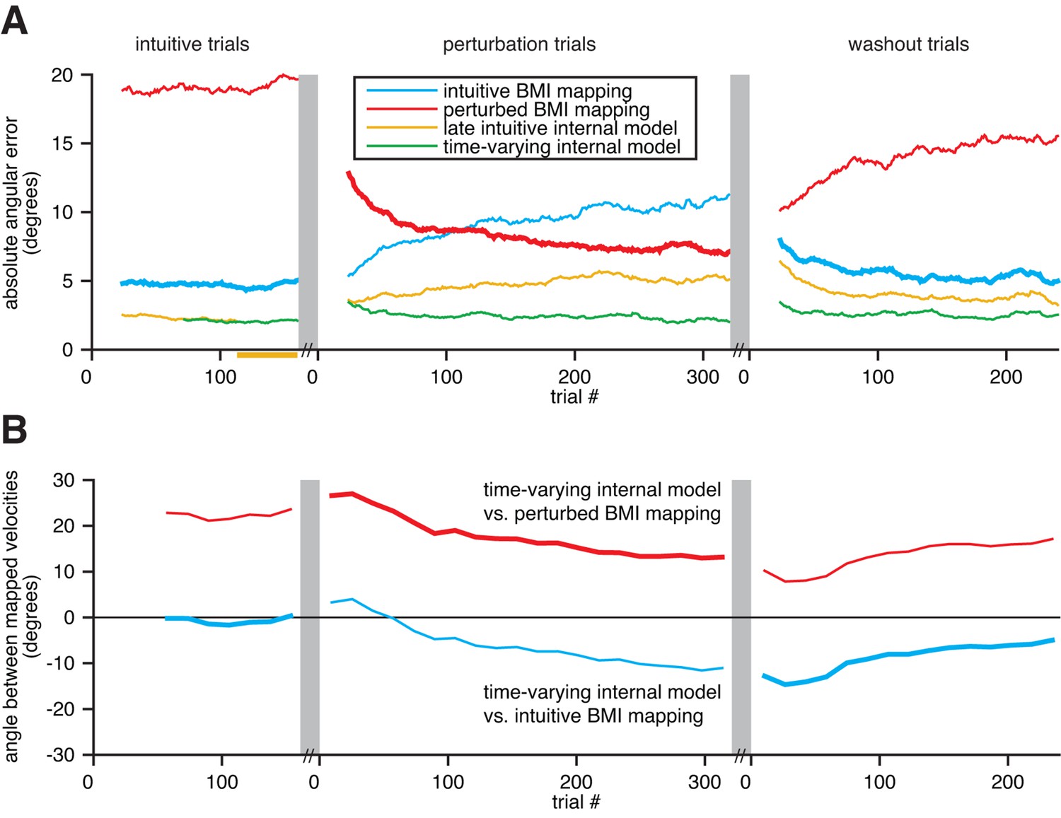
Extracted internal models capture adaptation to perturbations.
(A) Cross-validated angular errors computed by interpreting monkey A neural activity through BMI mappings and internal models. The intuitive BMI mapping (blue) defined cursor behavior during the intuitive and washout trials. The perturbed BMI mapping (red) defined cursor behavior during the perturbation trials. The late intuitive internal model (yellow) was extracted from the last 48 intuitive trials (yellow bar). A time-varying internal model (green) was extracted from a moving window of the 48 preceding trials. Values were smoothed using a causal 24-trial boxcar filter and averaged across 36 experiments. (B) Differences between monkey A’s time-varying internal model and the BMI mappings, assessed through the high-dimensional neural activity. For each round of 16 trials, neural activity from those trials was mapped to velocity through the time-varying internal model, the intuitive BMI mapping, and the perturbed BMI mapping. Signed angles were taken between velocities computed through the time-varying internal model and the intuitive BMI mapping (blue) and between velocities computed through the time varying internal model and the perturbed BMI mapping (red). Values were averaged across 36 experiments.
Download links
A two-part list of links to download the article, or parts of the article, in various formats.
Downloads (link to download the article as PDF)
Open citations (links to open the citations from this article in various online reference manager services)
Cite this article (links to download the citations from this article in formats compatible with various reference manager tools)
Internal models for interpreting neural population activity during sensorimotor control
eLife 4:e10015.
https://doi.org/10.7554/eLife.10015


