Cellular coordination underpins rapid reversals in gliding filamentous cyanobacteria and its loss results in plectonemes
- School of Life Sciences, University of Warwick, United Kingdom
- Department of Physics and Astronomy, University of Padova, Italy
- School of Physics, University of Warwick, United Kingdom
- Departamento de Estructura de la Materia, F´ısica Termica y Electronica, Facultad de Ciencias F´ısicas, Universidad Complutense de Madrid, Spain
- Instituto Mediterr´aneo de Estudios Avanzados, IMEDEA, Spain
Figures
Figure 1 with 5 supplements
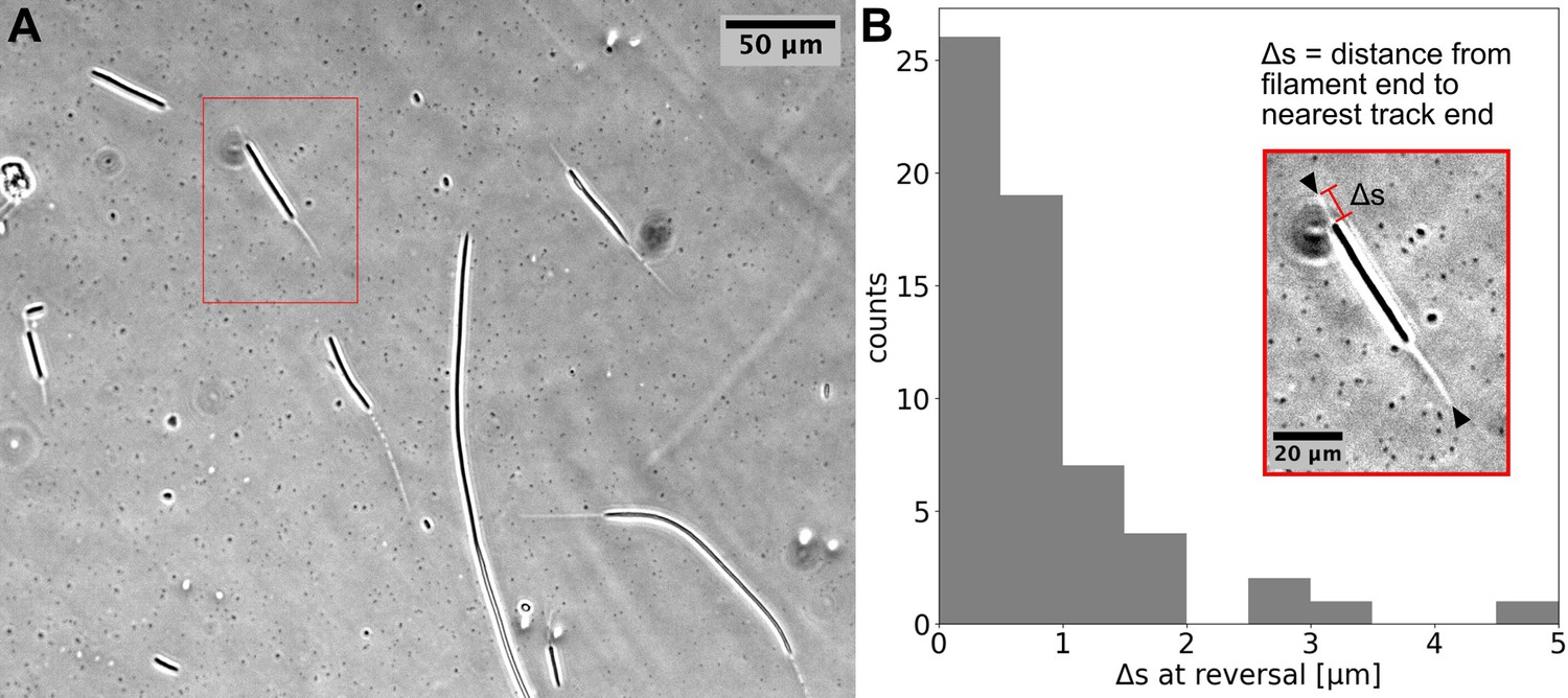
Cyanobacterial filaments move on `tracks’ on agar.
(A) Phase contrast image of filaments on an agar pad, showing `tracks' associated with moving filaments. (B) Distribution of distance between the end of the filament and the closest track end () at reversals (see Inset). Data is from multiple filaments (), each showing several reversals, resulting in 61 data points. Approximately 70% ~of the values are less than the measurement error (≈1). Inset: the single filament and track highlighted in (A) with a red box. Track ends are indicated by black arrowheads.
Figure 1—figure supplement 1
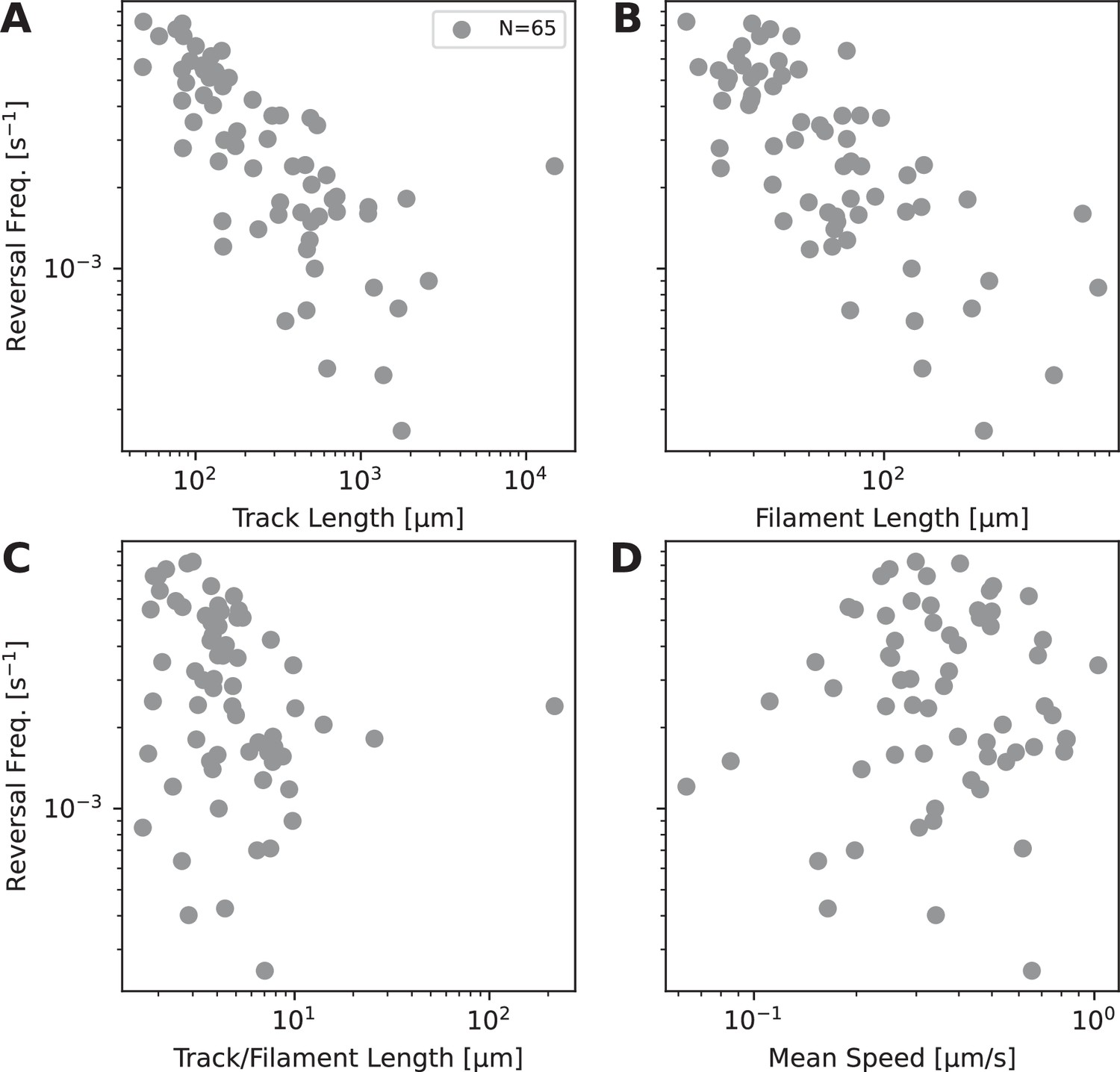
Reversal frequency as a function of different variables.
(A). Reversal frequency against track length, determined from extreme boundaries of filament movement during observation time. Data collected from 65 filaments observed as moving under agar. (B). Reversal frequency against filament length. (C). Reversal frequency against filament length normalised by track length. (D). Reversal frequency against filament mean speed.
Figure 1—video 1
Filament moving under 1.5% agarose sandwich.
Magnification of ×4 (1.61µm/pixel). Time interval of 5 s. Fluorescence recorded in Red channel with 100ms exposure. AVI produced with 20 fps compression.Link: https://youtu.be/RsANG2RBzTg.
Figure 1—video 2
Single filament in track on 2.5% agarose.
Magnification of 10 (0.645 μm/pixel). Time interval of 5 seconds. Phase image with 5 ms exposure. AVI produced with 20 fps compression. Link: https://youtu.be/XVIv4FLYBas.
Figure 1—video 3
Single filament on a circular trajectory on 1.5% agarose.
Magnification of 4 (1.61 μm/pixel). Time interval of 5 s. Fluorescence recorded in the Red channel with 100 ms exposure. AVI produced with 20 fps compression. https://youtu.be/PJdFEE6R6fk.
Figure 1—video 4
Several filaments in track on 2.5% agarose.
Magnification of 10 (0.645 μm/pixel). Time interval of 5 s. Phase image with 5 ms exposure. AVI produced with 20 fps compression. Link: https://youtu.be/hu-U810RMuw.
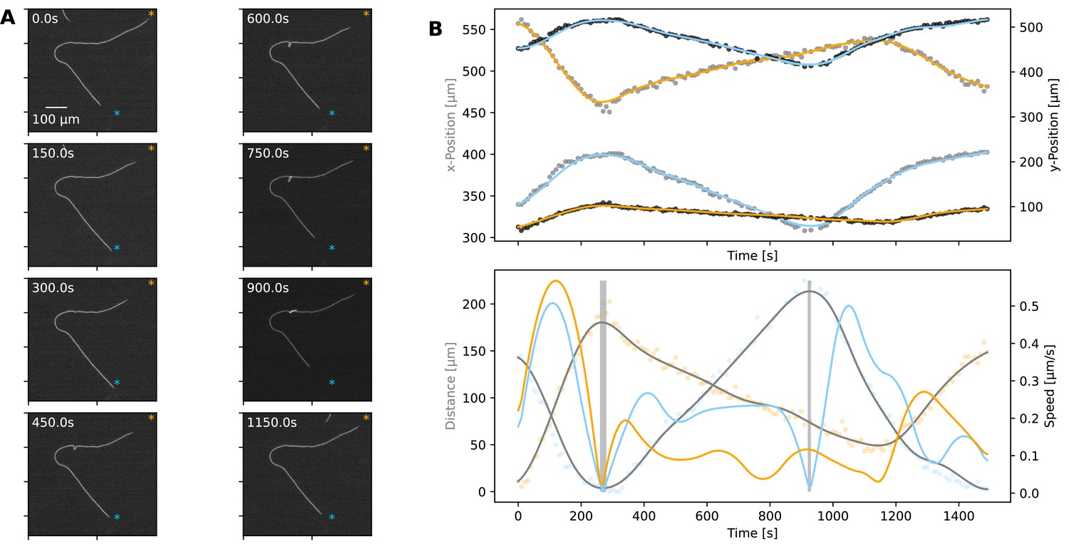
Figure 2 with 5 supplements
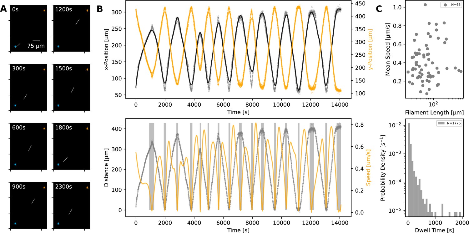
Statistics of filament motion on agar.
(A) A single filament shown at different time points of its movement under an agar pad. Time-lapse images were captured at 2 s intervals using fluorescence microscopy. The scale bar shown on the first image applies to all subsequent ones. The extreme points of the trajectory across the time lapse are marked with blue and orange asterisks on each image. (B) Top: X- and Y-coordinates of the filament’s centre throughout the recorded time-lapse. The points show observations, while the line shows a spline fit to this data. Bottom: The distance (grey) between filament centre and one of the extreme ends of its trajectory, shown with blue asterisk on panel A, and filament speed (orange) throughout the time-lapse. The speed is calculated from the spline fitted to the x- and y-coordinates shown in the top panel. Grey backdrop regions indicate time points with speed below a set threshold, indicating reversal events. (C) Top: Mean filament speed from 65 different filaments observed under agar, plotted against filament length. Bottom: Distribution of dwell times, as calculated from independent reversal events. For the same analyses for observations on glass, see (Figure 2—figure supplement 2).
Figure 2—figure supplement 1
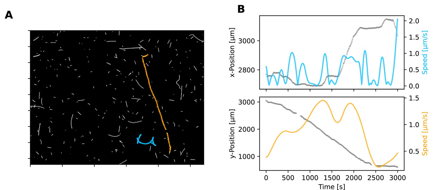
Example filament trajectories on glass.
(A) Single frame from a movie, showing filaments on glass (this image is associated with Figure 2—video 1). Two selected filaments are highlighted with their trajectories, coloured in blue and orange. (B) Trajectory (blue and orange) and speeds (grey) of filaments shown in panel A. Trajectory colours are matching to panel A. Trajectories are only shown in terms of either the x- or y-axis for simplicity, with the axis of the most significant movement shown.
Figure 2—figure supplement 2
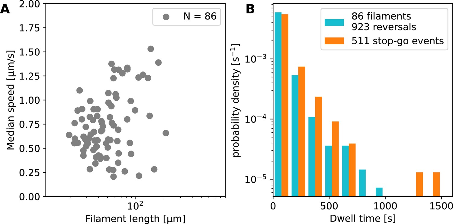
Summary statistics for filament motion on glass.
(A) Median speed against mean filament length for filaments moving on glass. Data from 86 individual filaments. There is a weak positive correlation between filament speed and length, which supports the conclusion that multiple (or all) cells contribute to propulsion. (B) Distribution of dwell times (the duration of stopping events) for movement on glass. On glass, we observe an additional behaviour following a stopping event, where the filament continues in the same direction instead of reversing, which we call a ‘stop-go’ event. The dwell time histograms for the reversals (blue) and the stop-go (orange) events are similar in shape, and there are approximately twice as many reversals as stop-go events.
Figure 2—figure supplement 3
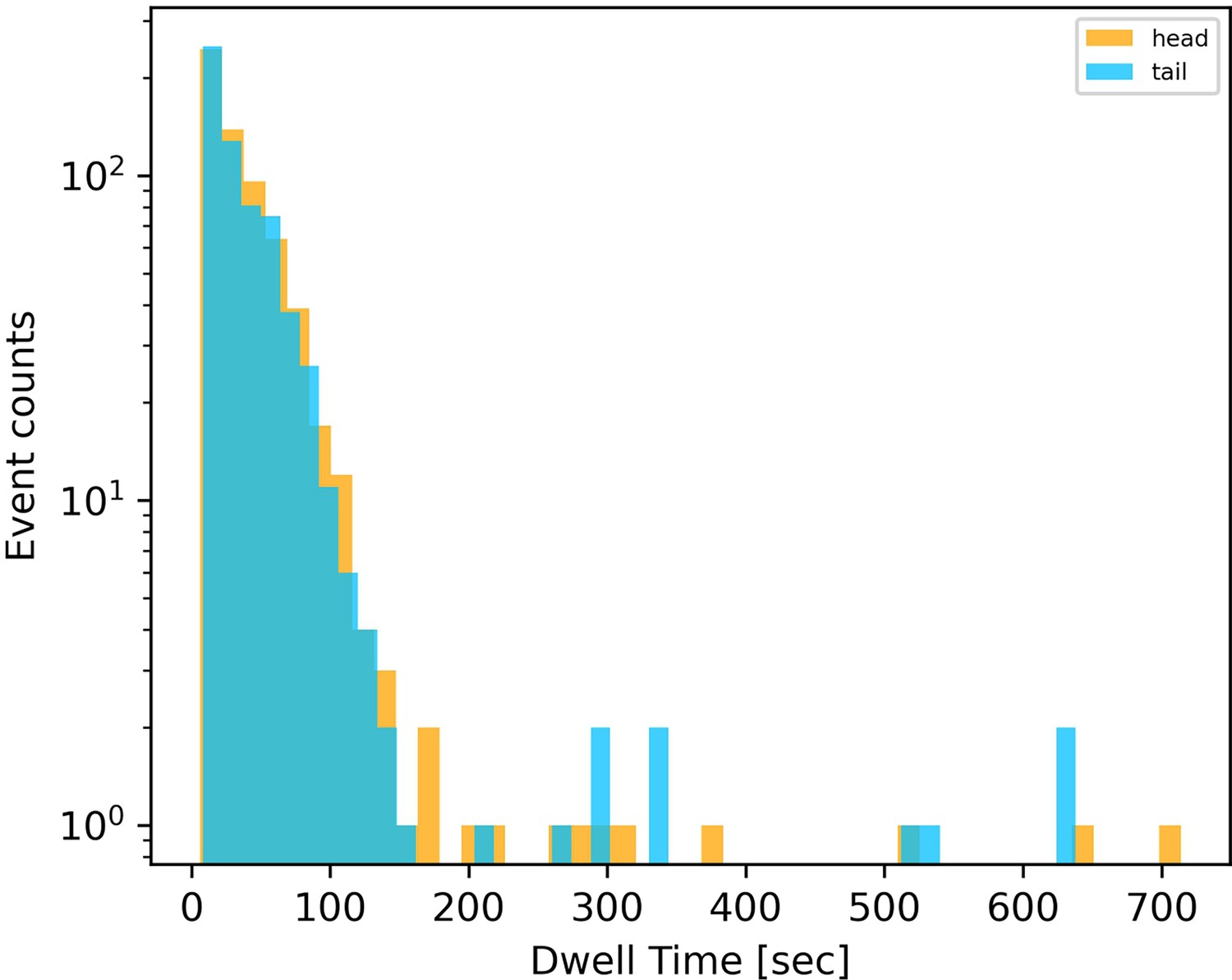
Distribution of dwell times of leading (head) and trailing (tail) ends of filaments.
Data is collated from 632 reversal events across 65 filaments. Only those reversals where dwell times estimated from tracking filament ends differed by less than a threshold from those estimated from filament centre, are included.
Figure 2—figure supplement 4
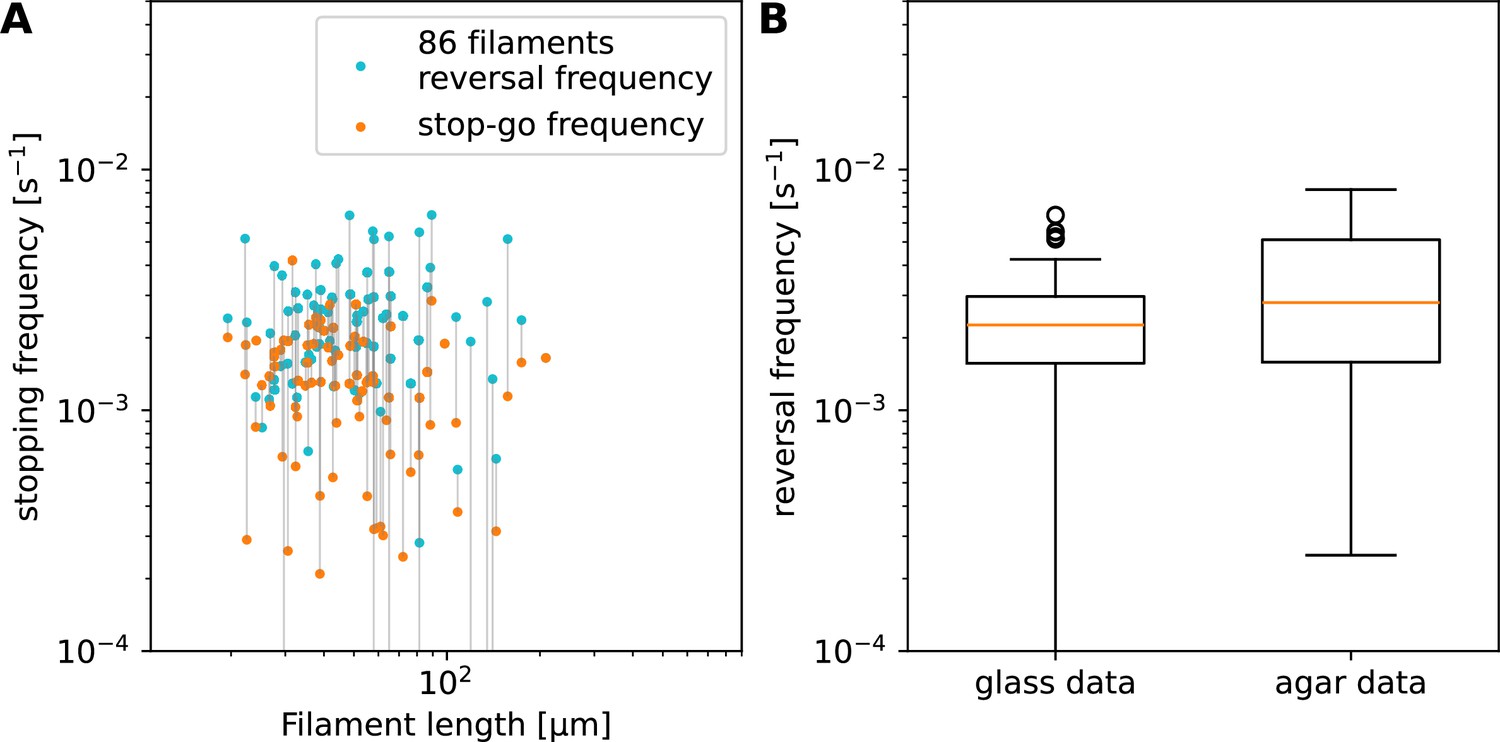
Summary statistics for stopping frequency.
(A) Reversal and stop-go frequency as a function of filament length on glass, split up for each filament into ‘stop-reverse’ (blue) and ‘stop-go’ (orange) events, depending on the direction of motion following the stopping event. The two points for each individual filament are joined by grey lines (note that some of the lines are not connected, due to some filaments analysed showing either no reversals or no stop-go events, over the entire track, giving a frequency of 0 for those points, which are therefore undefined on this logarithmic axis.) The reversal frequency is generally higher than the stop-go frequency. Frequencies are approximately constant with filament length, with an average of one reversal every 410 s, in contrast to the agar data. (B) Distribution of reversal frequency data from observations on glass and agar. On agar, the highest reversal frequencies (mostly observations from shorter filaments/tracks) are higher than the average on glass, while the lowest frequencies (mostly due to longer filaments/tracks) are comparable to the lower glass values. This corroborates the hypothesis that on agar, the reversals are caused by the track ends, so that shorter filaments are forced by the short tracks to reverse more often than their intrinsic reversal frequency (suggested by the glass data).
Figure 2—video 1
Filaments moving across glass slide.
Magnification of 10 (0.645 μm/pixel). Time interval of 10 s. Fluorescence recorded in Red channel with 200 ms exposure. AVI produced with 20 fps compression. Link: https://youtu.be/KOcwKboCFZg.
Figure 3 with 9 supplements
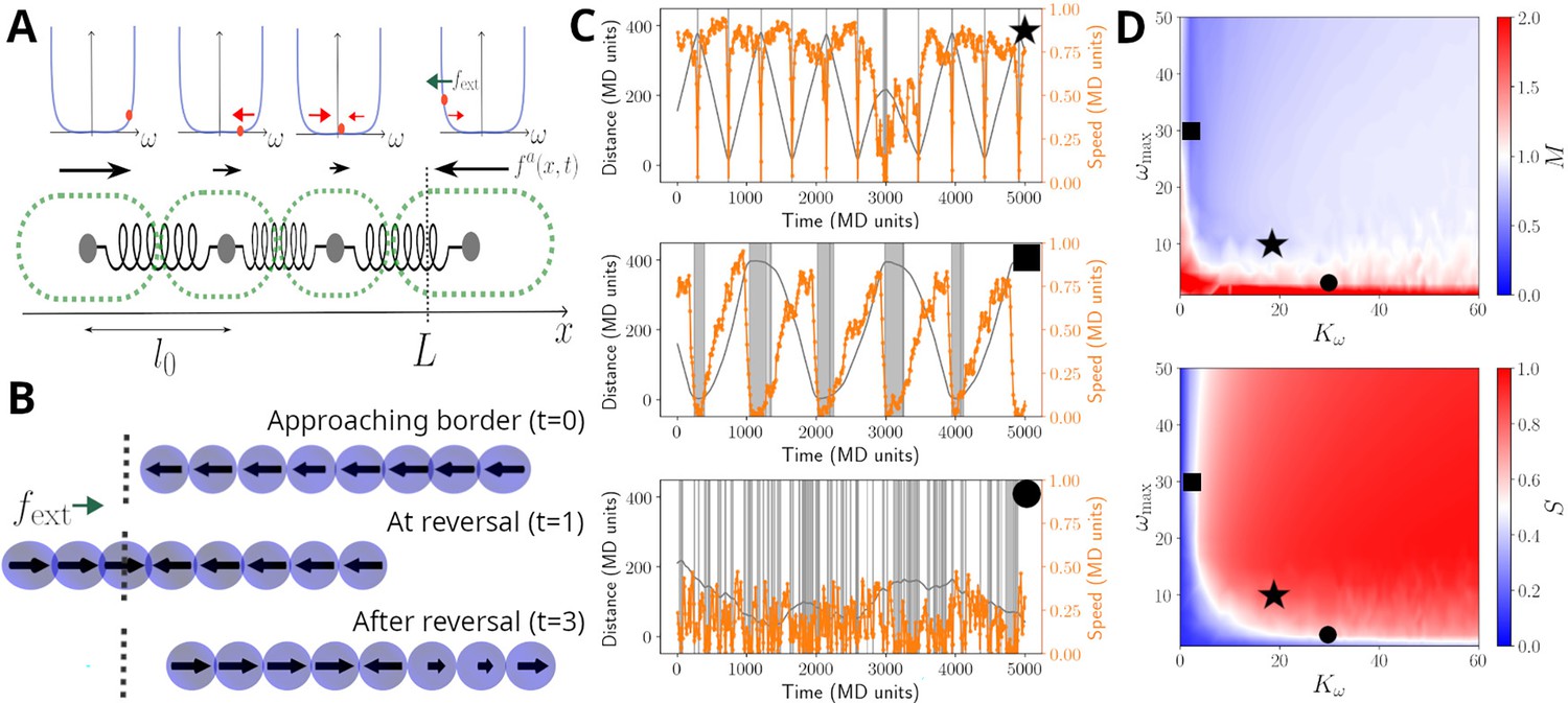
Model sketch, examples, and performance.
(A) A cartoon of the biophysical model (see Materials and methods). Cells are modelled as beads, connected by springs, with preferred rest length . Cells self-propel with a propulsion force . It is assumed that cells regulate the direction of , and this regulation is modelled by a function , which includes a self-regulatory element, implemented as a confining potential (shown as blue lines in the panels above cells). The value of each cell is represented with an orange dot, and it's affected by random fluctuations, a mechanical feedback from neighbouring cells (, red arrows), and an external signal , present at the ends of the track (green arrow; see Equation 5). (B) Example of reversal process: the snapshots show a coordinated filament approaching the border (top); after reaching it, the closest cells reverse their propulsion under the action of (centre). This prompts the rest of the cells to reverse and the filament coordinates again to travel in the opposite direction (bottom). (C) Simulated trajectories (grey lines) and absolute speed value (orange lines) as a function of time, presented as in Figure 2B, for units in a track of length . The different panels display a typical trajectory for a well-behaved filament (top, , ), a filament with little cell-to-cell coupling (centre, , ) or with little memory (bottom, , ). The grey bands highlight reversal events and their duration. (D) Contour plots of the synchronisation S (top) and of the reversal efficiency M (bottom) as a function of the cell-to-cell coupling and of the cell memory . See Materials and methods section for the definition of S and M. Black symbols highlight the systems showcased in panels (C).
Figure 3—figure supplement 1
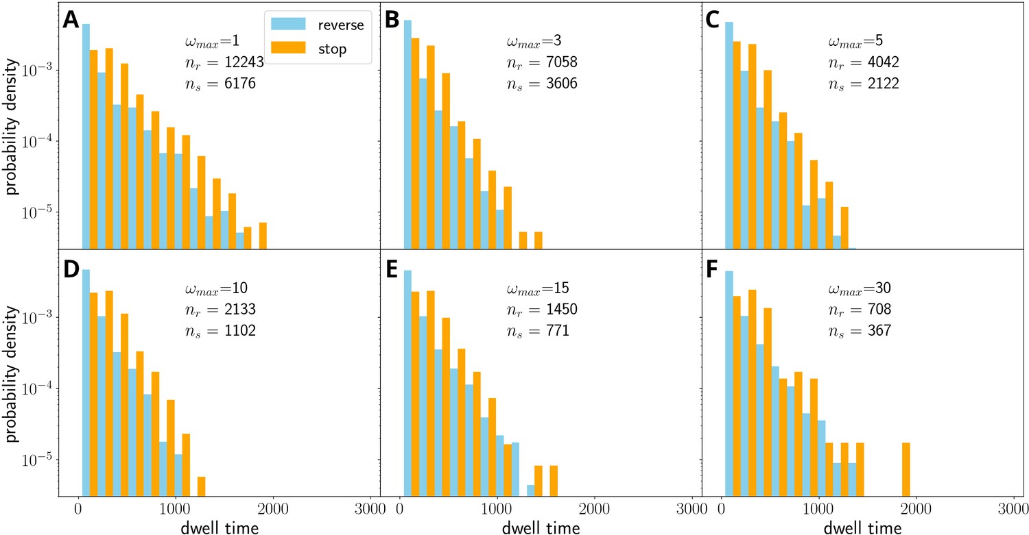
Distribution of stop/dwell times for simulated filaments on ‘glass’, that is without external forces.
We combine data from filaments with (as in Figure 2—figure supplement 2B), use a constant and different values of . Notice that, without coupling the cells' propulsion (=0, panel (A)), the distribution of dwell times develops a peak at some finite dwell time, and its tail becomes significantly fatter than in experiments. More importantly, the number of stop-go events becomes larger than the stop-reverse events, which does not match the experimental evidence. With increasing coupling (panels (B)-(D)), the distribution becomes markedly exponential, and the ratio between stop-go and stop-reverse instances matches the experimental value.
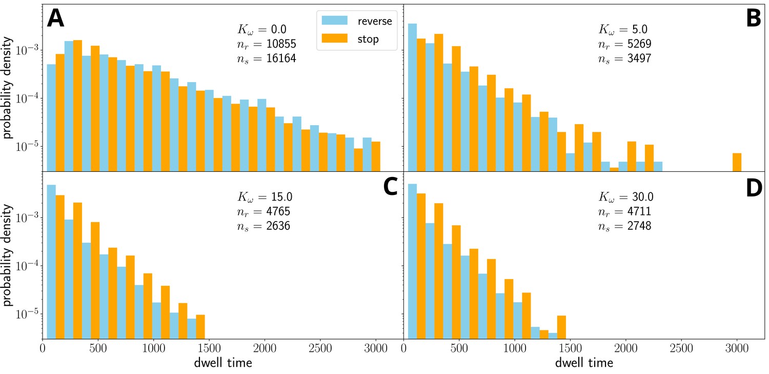
Figure 3—figure supplement 2
Distribution of stop/dwell times for =100, and several values of , for simulations without external force field.
Above a certain threshold (panels (B)-(F)), the dwell time distribution is independent of the parameter . However, the number of stops or reversals decreases, as it is harder to de-coordinate the filament.
Figure 3—figure supplement 3
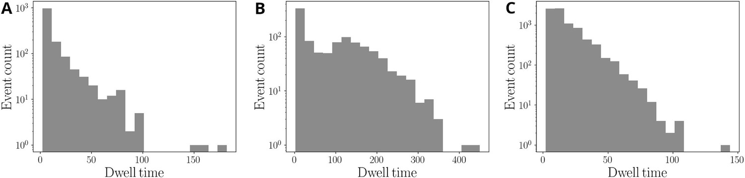
Simulated distribution of dwell times.
The parameters values are as in Figure 3C: (A) , ; (B) , ; (C) , .
Figure 3—figure supplement 4
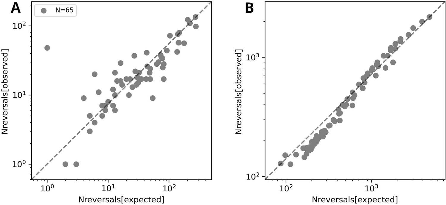
Number of reversals against the number of expected reversals as observed in experiments under agar (A) or in simulations (B).
One outlier filament in the experimental data involved reversals prior to track ends, but in a consistent location in the track. Simulated data have been obtained with and and several different values of .
Figure 3—figure supplement 5
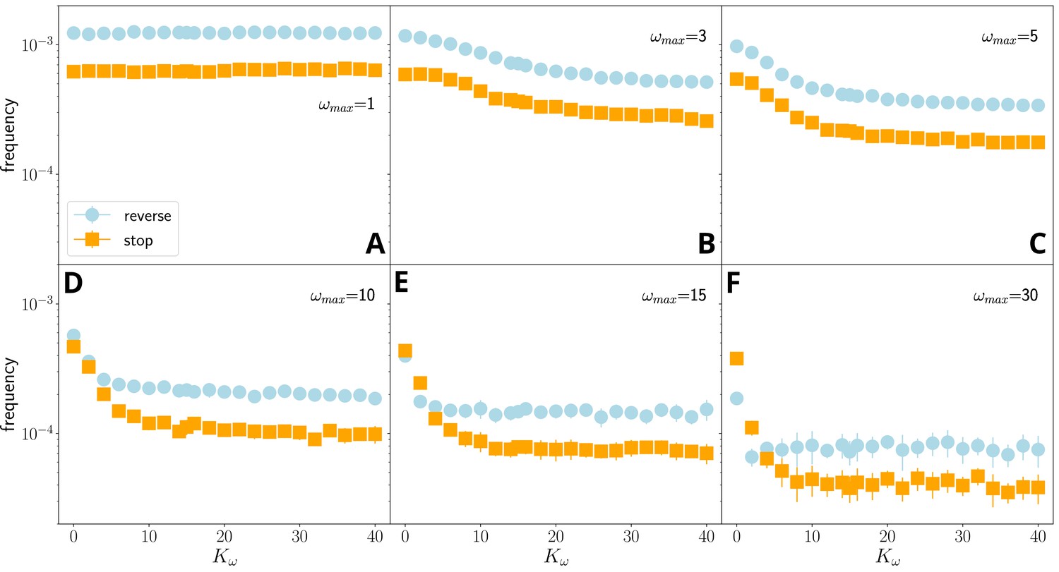
Average reversal frequency for stop-reverse (blue) and stop-go (orange) events as a function of for and different values of memory parameter, , for simulations without external force field.
At very small values of ((A), negligible memory), the frequencies of stops and reversals do not depend on , that is, the filament is not coordinated. With increasing ((B)-(F)), the frequency decreases with increasing and .
Figure 3—figure supplement 6
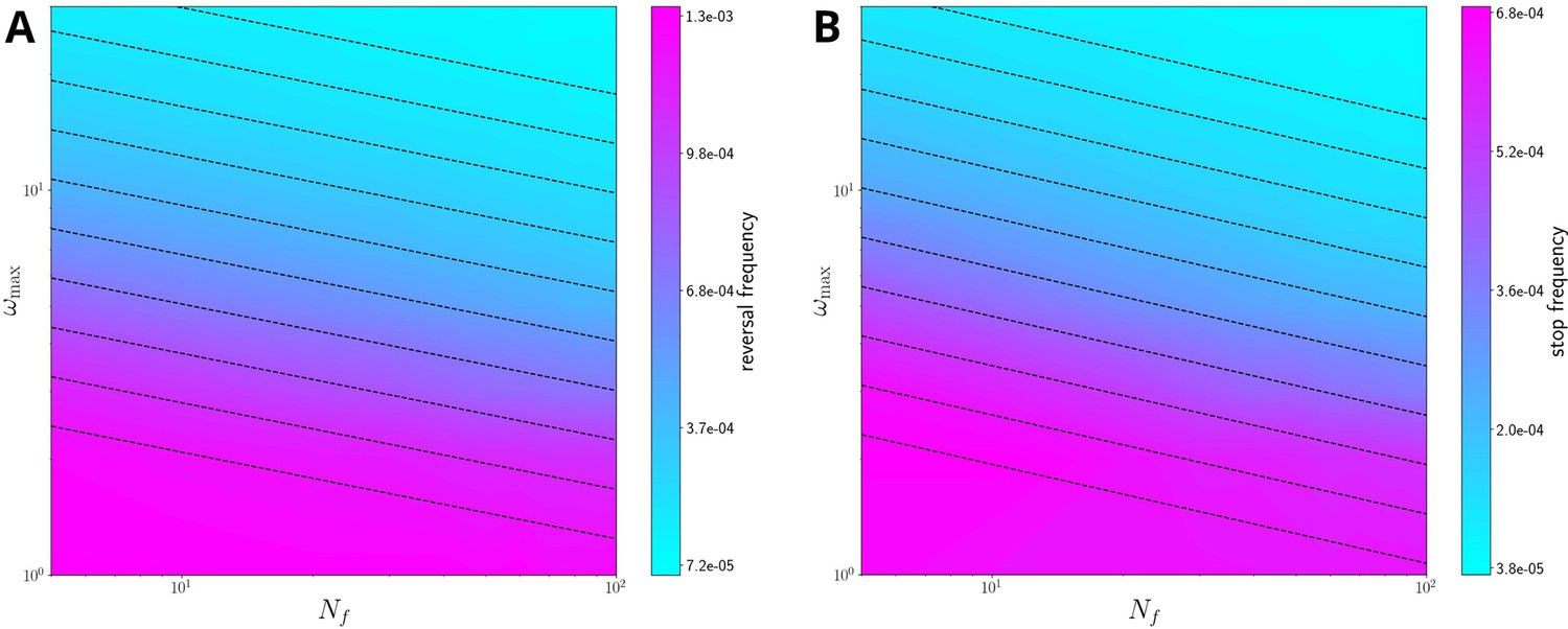
The relation of reversal frequency (A) and stop frequency (B) with filament length and memory parameter (i.e., in the plane) at fixed , for simulations without external force field.
Note that the reversal frequency is always higher than the stopping frequency. The black dashed lines are approximated level curves, obtained by fitting the relationship between and at fixed reversal/stopping frequency as a power law; in particular, we obtain the phenomenological relations for the reversal frequency and for the stopping frequency. The reversal frequency (A) and median filament velocity (B) against, and set using (at fixed = 15) for simulations without external field. Notice that the reversal frequency (left panel) remains roughly constant, while the median velocity decreases. This is a limitation of the model, which does not include any mechanism for reducing filament drag, which, as previously mentioned, would rationalize the weak positive correlation between filament velocity and length; however, it is consistent with the overall observation that longer filaments tend to be less coordinated. fig:S16.
Figure 3—figure supplement 7
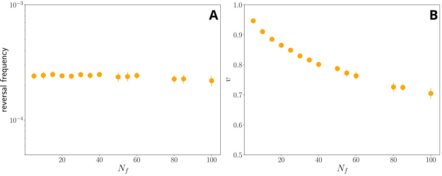
The reversal frequency (A) and median filament velocity (B) against Nf, and ωmax set using ωmax ∝ N−0.23 f (at fixed Kω=15) for simulations without external field.
Notice that the reversal frequency (left panel) remains roughly constant with Nf, while the median velocity decreases. This is a limitation of the model, which does not include any mechanism for reducing filament drag, which, as previously mentioned, would rationalize the weak positive correlation between filament velocity and length. However, it is consistent with the overall observation that longer filaments tend to be less coordinated.
Figure 3—video 1
Simulation movie of an active filament with a parameter set, resulting in coordinated reversals.
The filament is composed of 8 beads (cells) in a track of length 50 units. AVI produced with 5 fps compression. Link: https://youtu.be/nyUmk8QXz1I.
Figure 3—video 2
Simulation movie of an active filament with a parameter set, resulting in erratic reversals.
The filament is composed of 8 beads (cells) in a track of length 50 units. AVI produced with 5 fps compression. Link: https://youtu.be/Llc5oOmdxm0.
Figure 4 with 7 supplements
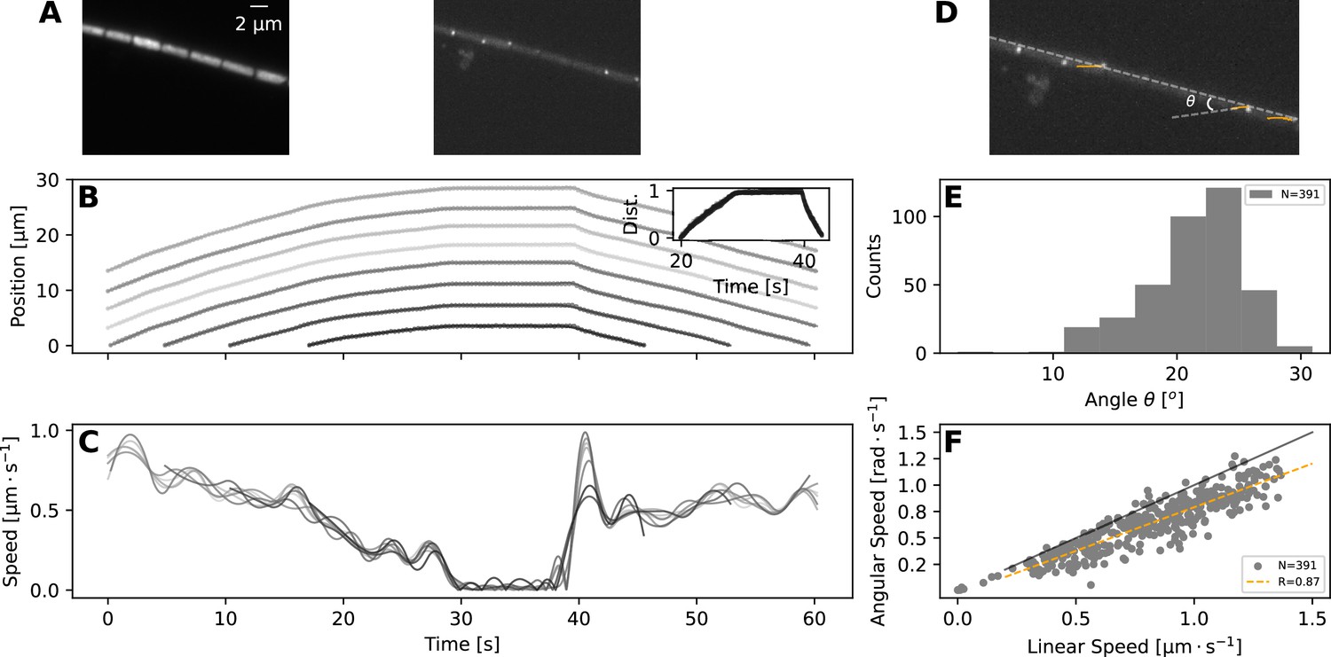
TIRF imaging reveals coupled rotation and translation.
(A) Individual images from a TIRF microscopy time-lapse, obtained with excitation using 473 nm laser. The left and right panel show images with emission filters centered at and , respectively. Note that these images show a thin (≈ 200nm) section of the cell membrane. (B,C) show respectively the position and speed of individual cells during this TIRF time-lapse movie (Figure 4—video 1). Different cells' trajectories and speed are shown in different shades of grey. The inset on panel (B) shows the normalised distance travelled by each cell, revealing high coordination in their movement. (D) The same TIRF image as shown on the right of (A), annotated with the trajectories of some of the membrane-bound protein complexes (orange lines) and the angle of this trajectory with the long axis of the filament; . (E,F) show respectively the distribution of the angle ; and the relation between rotational speed of the protein complexes and the linear speed of the filament. The black and orange lines in (F) show the expected diagonal and the correlation fit (see legend) between linear and angular speed. Both angle and speed measurements are collected from 11 filaments and 391 trajectories.
Figure 4—figure supplement 1
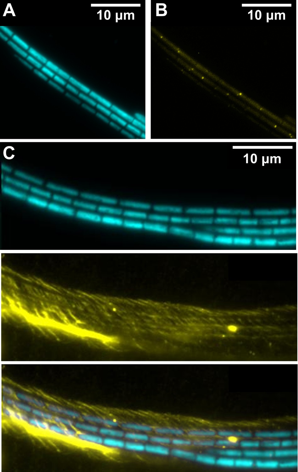
TIRF microscopy images of filament bundles.
(A) TIRF image of F. draycotensis filaments illuminated with light of wavelength 473 nm and imaged under an emission filter centred on 625 nm. (B) Same filaments under an emission filter centred on 525 nm, showing regularly placed fluorescent protein complexes. (C) TIRF image of a bundle of filaments stained using Concanavalin-A and illuminated with light of wavelength 473 nm. Top and middle panels show images with emission filters centred on 625 and 525 nm, respectively. Surrounding sheath of exopolysaccharide is visible (false coloured in yellow). The third panel shows the composite of these two emission channels.
Figure 4—figure supplement 2
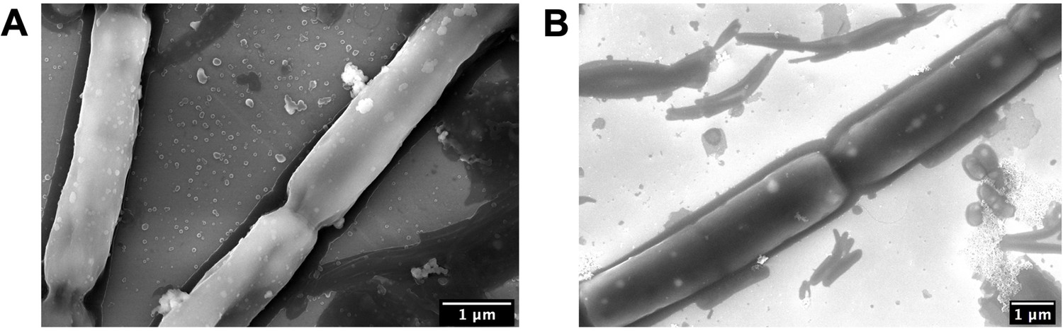
Scanning electron microscopy (SEM) images of the F. draycotensis cyanobacteria filaments.
(A) cyanobacteria filaments without further treatment, Mag.: ×40 k, EHT: 8 kV; (B) filaments following plasma cleaning inside SEM chamber, Mag.: ×25 k, EHT: 8 kV. Performed on a Zeiss Gemini, imaged on silicon wafer.
Figure 4—figure supplement 3
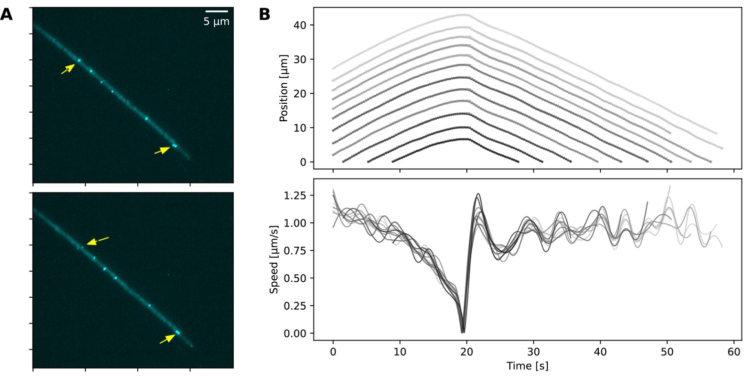
De-coordinated dynamics following reversal.
(A) Two time points in the movement sequence of a filament, the position and speed data for which is shown in panel B. The location of two protein complexes is shown with arrows, indicating that the complex further up the filament starts its movement earlier than the one at the tip of the filament. See also the associated Figure 4—video 3. (B) The position (top) and speed (bottom) of individual cells. Different cells' trajectories and speed are shown in different shades of grey.
Figure 4—figure supplement 4
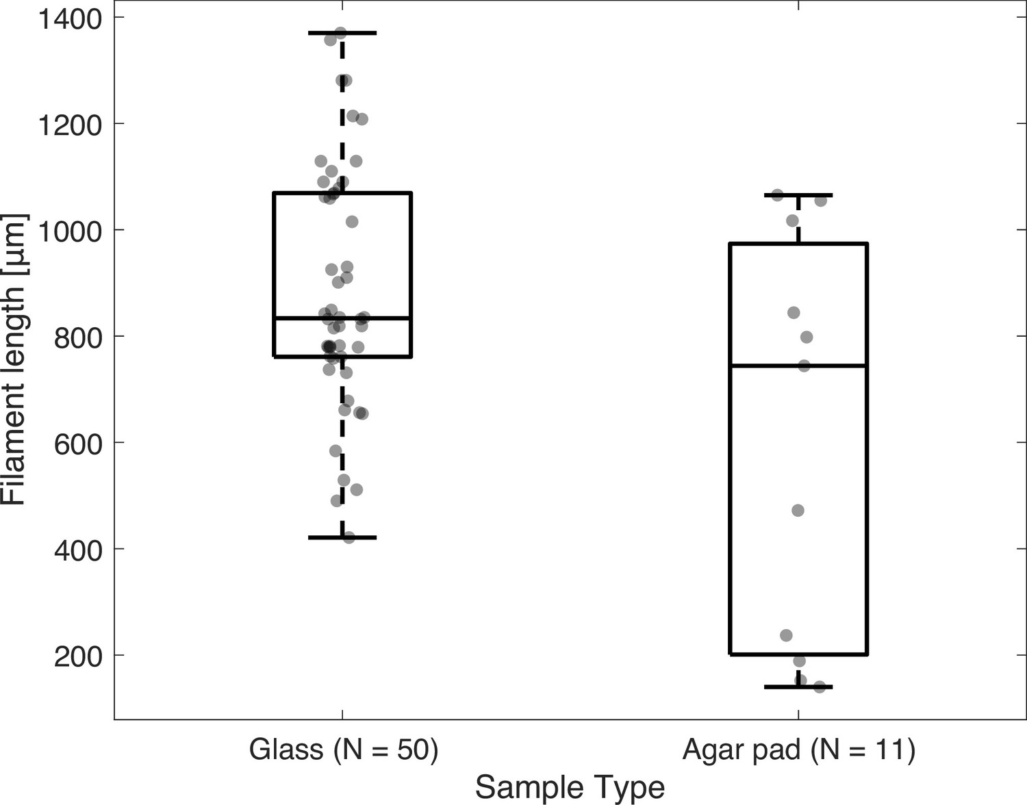
Distribution of filament lengths that exhibit buckling or plectonemes, shown for filaments observed on a glass slide (n=50), or sandwiched under agar (n=11).
Figure 4—video 1
TIRF imaging of a filament undergoing a reversal.
This shows the event analysed in Fig. 4. Magnification of ×100 (0.116 µm/pixel). Time interval of 33 ms. Fluorescence in cyan is from the bundled complexes on the filament surface, observed between 500-560 nm, with 30 ms exposure from a 473 nm laser. Fluorescence in the red channel comes from chlorophyll fluorescence, with 30 ms exposure from a 473 nm laser and observed in a channel between 600-670 nm. AVI produced with 100 fps compression. Link: https://youtu.be/Doa-jOkl04I.
Figure 4—video 2
TIRF imaging of stacked filaments in a stained slime sheath.
Magnification of ×100 (0.116 µm/pixel). Time interval of 33 ms. A 473 nm laser with an exposure time of 30 ms was used for excitation. The slime sheath is stained with concanavalin AlexaFluor-488 and coloured in yellow (observed 500-560 nm). Chlorophyll autofluorescence is coloured in cyano (observed 600-670 nm). AVI produced with 60 fps compression. Link: https://youtu.be/mYoqSqK9re0.
Figure 4—video 3
TIRF imaging of a filament undergoing a reversal, where fluorescence shows the protein complexes on the surface.
This movie is associated with the analysis shown in Figure 4—figure supplement 3. Magnification of ×100 (0.116 µm/pixel). Time interval of 33 ms. Fluorescence observed between 500-560 nm, with 30 ms exposure from a 473 nm laser. AVI produced with 100 fps compression. Link: https://youtube.com/shorts/pa5iIcua8Ps?feature=share.
Figure 5 with 3 supplements
Plectoneme formation.
(A) A filament forming a plectoneme during movement under agar, shown at different time points as indicated on each panel. (See Figure 5—video 1 for full video.) The scale bar shown on the first image applies to all subsequent ones. The orange and blue asterisks indicate the end-points of the filament’s trajectory. (B) Top: The x- and y-coordinates of the two ends of the filament over time. Data points for the x- and y-coordinates are shown in grey and black, respectively. Lines are spline fits to the data, and their orange and blue colours indicate the filament end that stays close to the corresponding trajectory end-point shown on the images in panel A. Bottom: Speed and distance of each end, respective to the end-point of the trajectory close to them. Speed is shown as blue and orange lines, calculated from the respective position data shown in the top panel. Distance is shown in orange and blue data points, indicating the filament end that stays close to the corresponding trajectory end-point shown on the images in panel A, while grey lines show spline fits. The shaded areas indicate the reversals. Note that the second reversal involves only the end that stays close to the blue asterisk on panel A.
Figure 5—video 1
Buckling filament under 1.5% agarose.
This video shows the event shown in Fig. 5. Magnification ×4 (1.61 µm/pixel). Time interval of 5 seconds. Fluorescence recorded in the Red channel with 100 ms exposure. AVI produced with 20 fps compression.Link: https://youtu.be/EmfIGJiiWUg.
Figure 5—video 2
Filament twisted in the middle, forming plectonemes on glass.
Magnification of ×4 (1.61 µm/pixel). Time interval of 30 s. Fluorescence recorded in Red channel with 100 ms exposure. AVI produced with 20 fps compression. Link: https://youtu.be/VzHMagiGqfo.
Figure 5—video 3
Filaments forming plectonemes on glass.
Magnification of ×4 (1.61 µm/pixel). Time interval of 5 s. Fluorescence recorded in Red channel with 100 ms exposure. AVI produced with 20 fps compression. Link: https://youtu.be/OBm0IpUN6rI.
Additional files
Download links
A two-part list of links to download the article, or parts of the article, in various formats.
Downloads (link to download the article as PDF)
Open citations (links to open the citations from this article in various online reference manager services)
Cite this article (links to download the citations from this article in formats compatible with various reference manager tools)
Cellular coordination underpins rapid reversals in gliding filamentous cyanobacteria and its loss results in plectonemes
eLife 13:RP100768.
https://doi.org/10.7554/eLife.100768.3


