Extracting grid cell characteristics from place cell inputs using non-negative principal component analysis
Figures
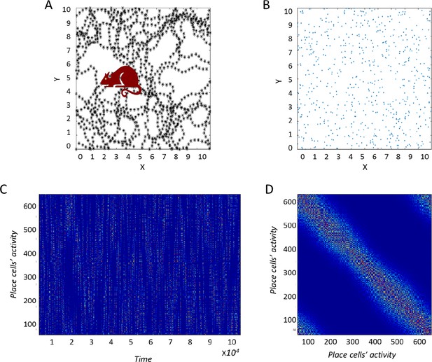
Construction of the correlation matrix from behavior.
(A) Diagram of the environment. Black dots indicate places the virtual agent has visited. (B) Centers of place cells uniformly distributed in the environment. (C) The [Neuron X Time] matrix of the input-place cells. (D) Correlation matrix of (C) used for the PCA process.
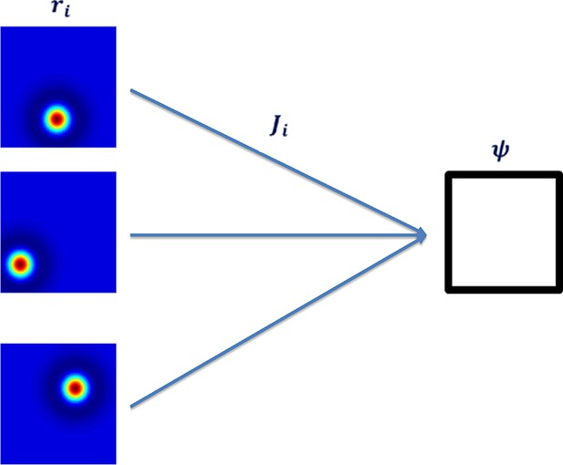
Neural network architecture with feedforward connectivity.
The input layer corresponds to place cells and the output to a single cell.
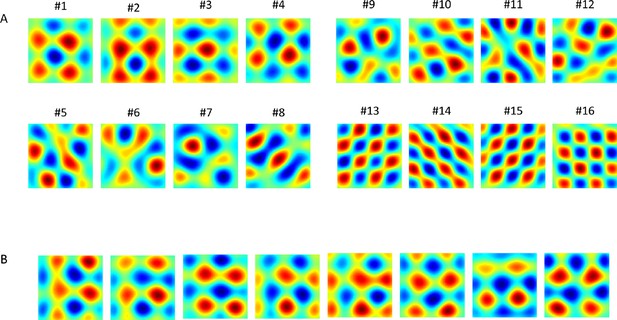
Results of PCA and of the networks' output (in different simulations).
(A) 1st 16 PCA eigenvectors projected on the place cells' input space. (B) Converged weights of the network (each result from different simulation, initial conditions and trajectory) projected onto place cells' space. Note that the 8 outputs shown here resemble linear combinations of components #1 to #4 in panel A.
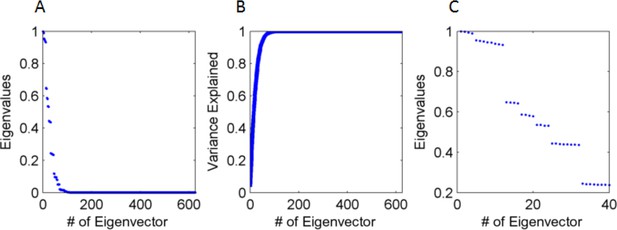
Eigenvalues and eigenvectors of the input's correlation matrix.
(A) Eigenvalue size (normalized by the largest, from large to small (B) Cumulative explained variance by the eigenvalues, with 90% of variance accounted for by the first 35 eigenvectors (out of 625). (C) Amplitude of leading 32 eigenvalues, demonstrating that they cluster in groups of 4 or 8. Specifically, the first four clustered groups correspond respectively (from high to low) to groups A,B,C & D In Figure 15C, which have the same redundancy (4,8,4 & 4).
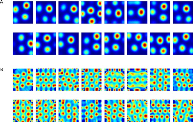
Output of the neural network when weights are constrained to be non-negative.
(A) Converged weights (from different simulations) of the network projected onto place cells space. See an example of a simulation in Video 1. (B) Spatial autocorrelations of (A). See an example of the evolution of autorcorrelation in simulation in Video 2.
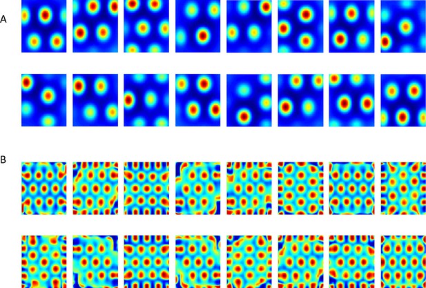
Results from the non-negative PCA algorithm.
(A) Spatial projection of the leading eigenvector on input space. (B) Corresponding spatial autocorrelations. The different solutions are outcomes of multiple simulations with identical settings in a new environment and new random initial conditions.
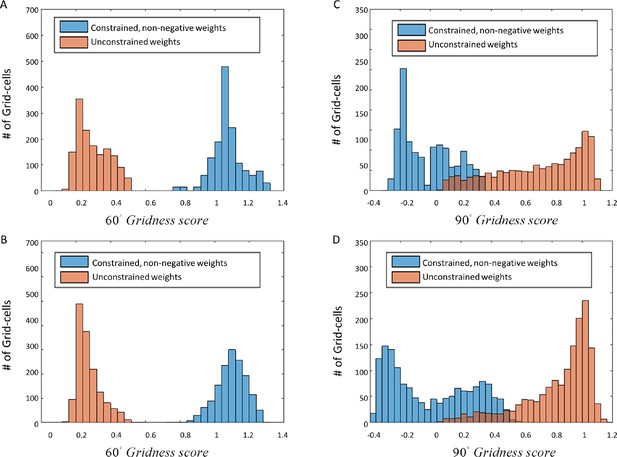
Histograms of Gridness values from network and PCA.
First row (A) + (C) corresponds to network results, and second row (B) + (D) to PCA. The left column histograms contain the 60° Gridness scores and the right one the 90° Gridness scores.

Different types of spatial input used in our network.
(A) 2D Gaussian function, acting as a simple place cell. (B) Laplacian function or Mexican hat. (C) A positive (inner circle) - negative (outer ring) disk. While inputs as in panel A do not converge to hexagonal grids, inputs as in panels B or C do converge.
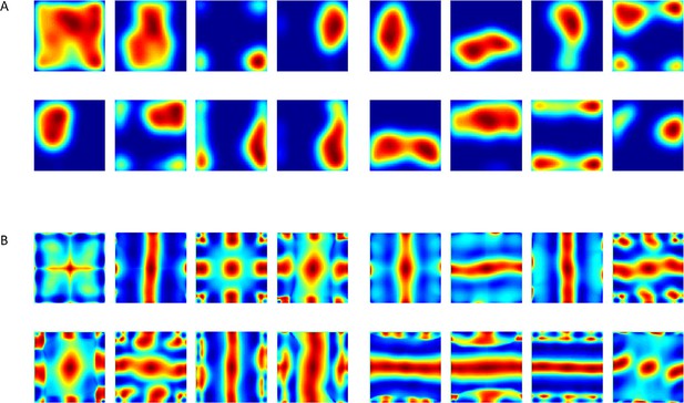
Spatial projection of outputs’ weights in the neural network when inputs did not have zero mean (such as in Figure 8A).
(A) Various weights plotted spatially as projection onto place cells space. (B) Autocorrelation of (A).
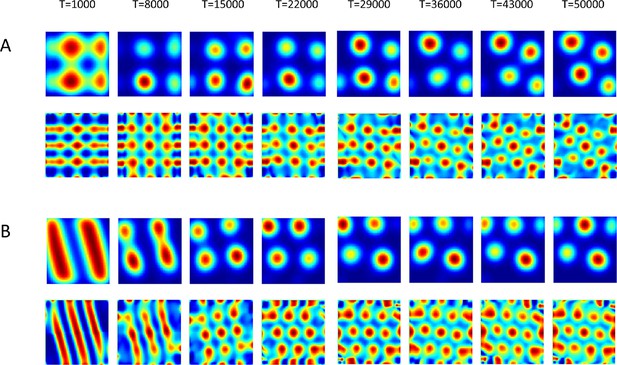
Evolution in time of the networks’ solutions (upper rows) and their autocorrelations (lower rows).
The network was initialized in shapes of (A) Squares and of (B) stripes (linear).
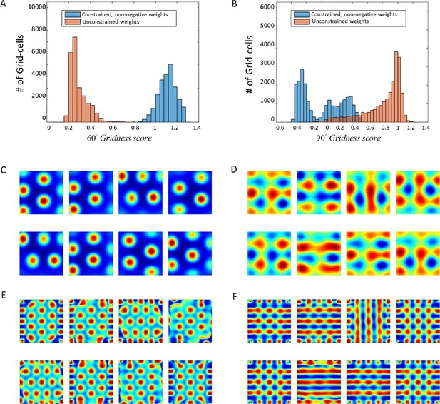
Numerical convergence of the ODE to hexagonal results when weights are constrained.
(A) + (B): 60° and 90° Gridness score histograms. Each score represents a different weight vector of the solution J. (C) + (D): Spatial results for constrained and unconstrained scenarios, respectively. (E) + (F) Spatial autocorrelations of (C) + (D).
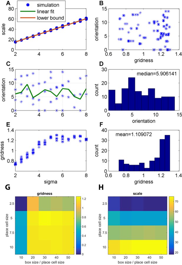
Effect of changing the place-field size in fixed arena (FISTA algorithm used; periodic boundary conditions and Arena size 500);
(A) Grid scale as a function of place field size (sigma); Linear fit is: Scale = 7.4 Sigma+0.62; the lower bound, equal to , were is defined in Equation 32 in the Materials and methods section; (B) Grid orientation as a function of gridness; (C) Grid orientation as a function of sigma – scatter plot (blue stars) and mean (green line); (D) Histogram of grid orientations; (E) Mean gridness as a function of sigma; and (F) Histogram of mean gridness. (G) Gridness as a function of sigma and (arena-size/sigma) (zero boundary conditions). (H) Grid scale for the same parameters as in G.
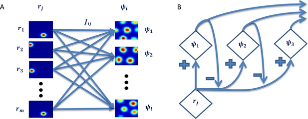
Hierarchial network capable of computing all 'principal components'.
(A) Each output is a linear sum of all inputs weighted by the corresponding learned weights. (B) Over time, the data the following outputs 'see' is the original data after subtration of the 1st 'eigenvector's' projection onto it. This is an iterative process causing all outputs' weights to converge to the 'prinipcal components' of the data.
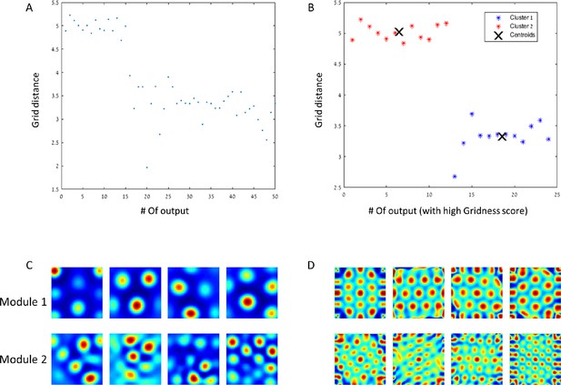
Modules of grid cells.
(A) In a network with 50 outputs, the grid spacing per output is plotted with respect to the hierarchical place of the output. (B) The grid spacing of outputs with high Gridness score (>0.7). The centroids have a ratio of close to . (C) + (D) Example of rate maps of outputs and their spatial autocorrelations for both of the modules.
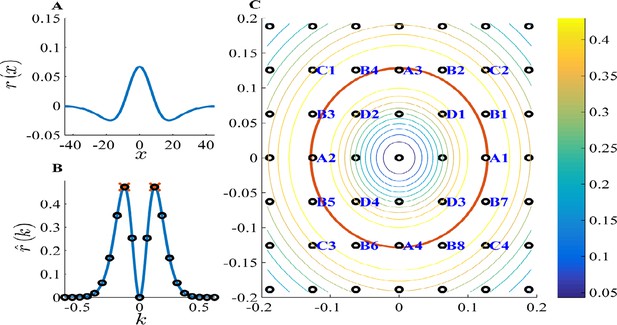
PCA k-space analysis for a difference of Gaussians tuning curve.
(A) The 1D tuning curve . (B) The 1D tuning curve Fourier transform . The black circles indicate k-lattice points. The PCA solution, , is given by the circles closest to , the peak of (red cross). (C) A contour plot of the 2D tuning curve Fourier transform . In 2D k-space the peak of becomes a circle (red), and the k-lattice is a square lattice (black circles). The lattice point can be partitioned into equivalent groups. Several such groups are marked in blue on the lattice. For example, the PCA solution Fourier components lie on the four lattice points closest to the circle, denoted A1-4. Note the grouping of A,B,C & D (4,8,4 and 4, respectively) corresponds to the grouping of the 20 highest principal components in Figure 4. Parameters: .
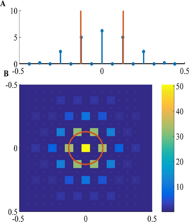
Fourier components of Non-negative PCA on the -lattice.
(A) 1D solution (blue) includes: a DC component (), a maximal component with magnitude near (red line), and weaker harmonics of the maximal component. (B) 2D solution includes: a DC component (k = (0,0)), a hexgaon of strong components with radius near (red circle), and weaker components on the lattice of the strong components. White dots show underlying -lattice. We used a difference of Gaussians tuning curve, with parameters , and the FISTA algorithm.
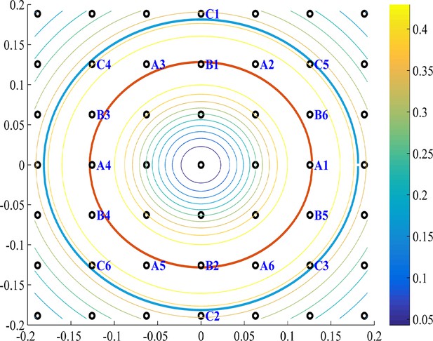
The modules in Fourier space.
As in Figure 15C, we see a contour plot of the 2D tuning curve Fourier transform and the k-space the peak of (red circle), and the k-lattice (black circles). The lattice points can be divided into approximately hexgonal shaped groups. Several such groups are marked in blue on the lattice. For example, group A and B are optimal since they are nearest to the red circle. The next best (with the highest-valued contours) group of points, which have an approximate hexgonal shape, is C. Note that group C has a k-radius of approximately the optimal radius times (cyan circle). Parameters: .
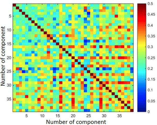
Demonstrates that output vectors are not orthogonal.
Matrix of cosine values between every two vectors.
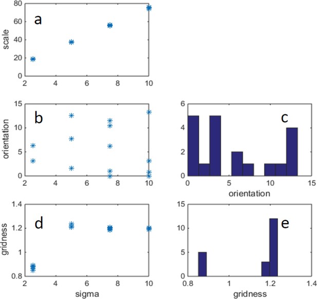
Example of changing width of place cells (σ) and correspondingly changing arena size, such that there is a fixed ratio: arena_size/σ = 40.
(FISTA algorithm was used for positive PCA, with 0 boundary conditions.) (a) Grid scale as a function of σ (place cell width); (b) Grid orientation as a function of σ. (c) Histogram of grid orientations (d) Mean gridness as a function of σ. (e) Histogram of mean gridness.
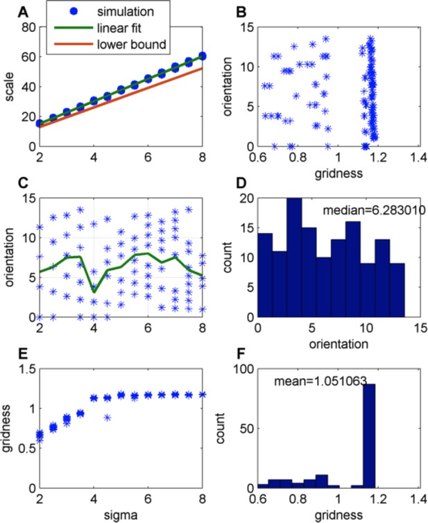
Effect of changing the place-field size in a constant boundary (FISTA algorithm used; zero boundary conditions and Arena size 500);
(A) Grid scale as a function of place field size (σ); Linear fit is: Scale = 7.4. Σ+0.62; the lower bound is equal to , where is defined in Eq. 32 in the Methods section; (B) Grid orientation as a function of gridness (green line is the mean); (C) Grid orientation as a function of σ – scatter plot (blue stars) and mean (green line); (D) Histogram of grid orientations; (E) Mean gridness as a function of σ; and (F) Histogram of mean gridness.
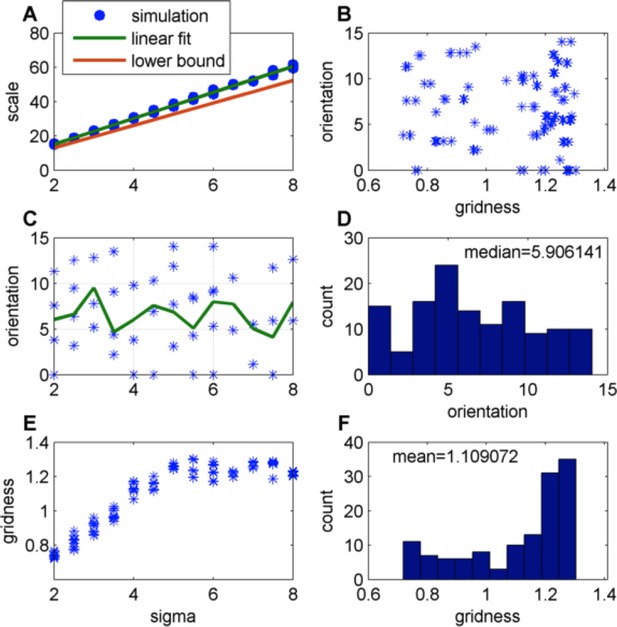
Effect of changing the place-field size in a constant boundary (FISTA algorithm used; periodic boundary conditions and Arena size 500);
(A) Grid scale as a function of place field size (σ); Linear fit is: Scale = 7.4 Σ+0.62; the lower bound, equal to , were is defined in Eq. 32 in the Methods section; (B) Grid orientation as a function of gridness; (C) Grid orientation as a function of σ – scatter plot (blue stars) and mean (green line); (D) Histogram of grid orientations; (E) Mean gridness as a function of σ; and (F) Histogram of mean gridness.
Videos
Evolution in time of the network's weights.
625 Place-cells used as input. Video frame shown every 3000 time steps up to t=1,000,000. Video converges to results similar to those of Figure 5.
Evolution of autocorrelation pattern of network's weights shown in Video 1.
https://doi.org/10.7554/eLife.10094.009Tables
List of variables used in simulation.
| Environment: | Size of arena | Place cells field width | Place cells distribution |
| Agent: | Velocity (angular & linear) | Initial position | ------------------- |
| Network: | # Place cells/ #Grid cells | Learning rate | Adaptation variable (if used) |
| Simulation: | Duration (time) | Time step | ------------------- |


